 Laue
Guide — Science
This guide is for crystallographers, physicists, chemists and mineralogists. It recalls the theoretical framework without detours, then states precisely what the Laue engine computes: the conventions, the models, their limits and their references. The formulas are open by default.
Documents, conventions and exactness
In Laue
A .laue document is a readable JSON file whose schema is published. It is identical on Mac, iPad and PC. The engine (LaueCore) computes everything that pertains to symmetry in exact rationals: operations, positions, Wyckoff coordinates. It switches to floating point for geometry, diffraction and refinement. A coordinate typed as 1/3 stays 1/3; a decimal value close to a simple fraction (0.33333) is snapped to it when a file is imported.
The conventions are those of the International Tables for Crystallography, Volume A: conventional cells, 530 settings described by their Hall symbol, Wyckoff letters and oriented site-symmetry symbols. The engine is checked against a battery of references: the operations of the 530 settings, the Wyckoff positions, the systematic absences and the powder patterns of known structures.
The Science usage in the settings gives the international and orbifold symbols, and brings diffraction to the fore.
Lattice, basis and metric tensor
Theory
A lattice is described, up to an isometry, by its metric tensor . This contains everything that does not depend on orientation: distances, angles, volume. The reciprocal lattice has metric . A change of basis transforms the coordinates by and the metric by . Miller indices transform like the basis, by ; coordinates transform contragrediently.
The fourteen Bravais types result from classifying lattices by their holohedry (the point group of the lattice) and their centring. The conventional cell is chosen so that the basis is adapted to this holohedry. The centring vectors (I: ½,½,½; F: ½,½,0 and permutations; C: ½,½,0; R in hexagonal axes: ⅔,⅓,⅓ and ⅓,⅔,⅔) belong to the translation group.
The formulas
In Laue
The Cell section exposes only the parameters left free by the crystal system of the group; the others are derived from them. Volume, distances and bonds are computed through . The setting of the group fixes the basis: for a monoclinic group, the choice of unique axis (b or c) and of cell (1, 2, 3); for a rhombohedral group, hexagonal (H) or rhombohedral (R) axes. Laue does not reduce the cell (no Niggli reduction): the cell is that of the chosen setting.
Point groups and Laue classes
Theory
The linear part of an operation that leaves a lattice invariant is, in a basis of that lattice, an integer matrix with determinant ±1. Its trace is therefore an integer, hence the crystallographic restriction: orders 1, 2, 3, 4 and 6 only. The finite subgroups of that respect it form 32 geometric classes. Eleven of them are centrosymmetric: these are the Laue classes, to which every diffraction pattern reduces in the absence of anomalous scattering (Friedel's law).
Neumann's principle requires every physical property tensor to be invariant under the point group. For example, piezoelectricity, a polar tensor of rank 3, vanishes in the 11 centrosymmetric classes and in class 432; pyroelectricity exists only in the 10 polar classes.
The formulas
Stereographic projection of a direction with colatitude and azimuth , onto the equatorial plane of the circle of radius :
In Laue
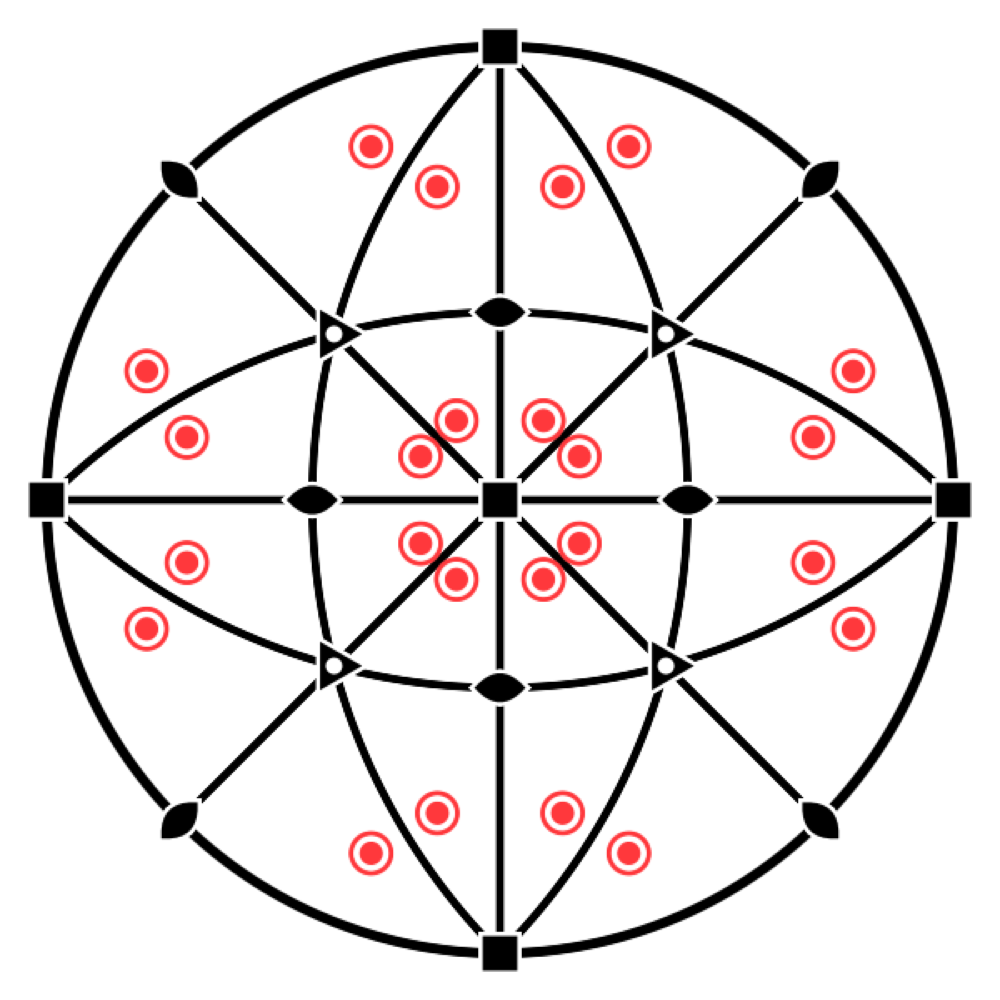
The Stereogram shows the point group with its elements and the orbit of a general direction (poles in the northern hemisphere as dots, southern as circles). When a site is selected, it shows its site-symmetry group, oriented in the cell. The crystal class is given in Hermann–Mauguin notation, with the system.
Space groups, Seitz and Hall
Theory
A space group is a discrete subgroup of the Euclidean group whose translation subgroup is a lattice. The quotient is isomorphic to the point group . is represented by coset representatives , or by 4 × 4 augmented matrices. The intrinsic translation part of an operation of order distinguishes a screw axis or a glide plane from a rotation axis or a mirror: it is computed by summing the powers of the operation. The remainder of is a location part, which fixes where the element lies.
The 230 space-group types are the equivalence classes under orientation-preserving affine changes of coordinate system: 219 affine types, including 11 enantiomorphic pairs (P4₁/P4₃, P3₁21/P3₂21…). The Hermann–Mauguin symbol names the type and its symmetry directions. The Hall symbol (Hall, 1981) gives an explicit set of generators in a given coordinate system, and therefore designates a setting unambiguously.
The formulas
Intrinsic part (glide or screw) of an operation of order , and location part:
The fixed points of give the location of the element: .
In Laue
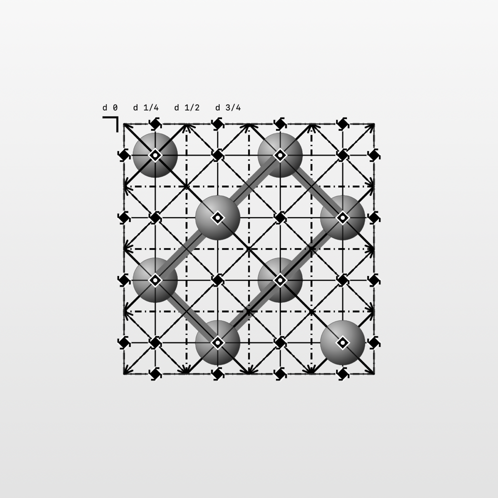
The group field accepts a number, a short or full HM symbol, a setting (227:1, 14:b2) or a Hall symbol (Hall: -P 2ybc). Each of the 530 settings is built from its Hall symbol. Symmetry elements are geometric objects in the sense of the Tables: an axis or a plane together with all the operations that share it, determined by the decomposition above. They are drawn with the graphical symbols of Volume A, and the Projection of the Tables reproduces its diagrams with the heights of the planes. The Orders filter isolates the axes of a given order.
The symbols of the Tables
What the Tables say
The diagrams of Volume A of the International Tables represent each symmetry element by a graphical symbol (section 1.4 of the 2006 edition, chapter 2.1 of the 2016 edition: they are the same). Laue draws these symbols in the 3D view, the projection of the Tables, the stereograms and the tilings; the figures in these tables come from the same library as the app. The notation is that of the Tables, with partial elements in parentheses; the intrinsic translation is given as a fraction of the shortest lattice translation along the axis or the glide.
Axes perpendicular to the drawing, symmetry points
| Symbol | Element | Notation | Intrinsic translation |
|---|---|---|---|
 | Twofold rotation axis; twofold point in the plane | 2 | — |
 | Screw axis 2₁ | 2₁ | |
 | Threefold rotation axis; threefold point in the plane | 3 | — |
 | Screw axis 3₁ | 3₁ | |
 | Screw axis 3₂ | 3₂ | |
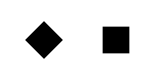 | Fourfold rotation axis; fourfold point in the plane | 4 (2) | — |
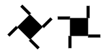 | Screw axis 4₁ | 4₁ (2₁) | |
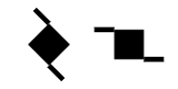 | Screw axis 4₂ | 4₂ (2) | |
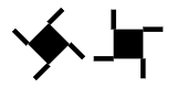 | Screw axis 4₃ | 4₃ (2₁) | |
 | Sixfold rotation axis; sixfold point in the plane | 6 (3, 2) | — |
 | Screw axis 6₁ | 6₁ (3₁, 2₁) | |
 | Screw axis 6₂ | 6₂ (3₂, 2) | |
 | Screw axis 6₃ | 6₃ (3, 2₁) | |
 | Screw axis 6₄ | 6₄ (3₁, 2) | |
 | Screw axis 6₅ | 6₅ (3₂, 2₁) | |
 | Inversion centre | — | |
 | Rotoinversion axis 3̄ | (3, ) | — |
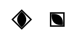 | Rotoinversion axis 4̄ | (2) | — |
 | Rotoinversion axis 6̄ | — | |
 | Twofold axis with an inversion centre | 2/m () | — |
 | Screw axis 2₁ with an inversion centre | 2₁/m () | |
 | Fourfold axis with an inversion centre | 4/m (, 2, ) | — |
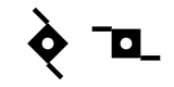 | Screw axis 4₂ with an inversion centre | 4₂/m (, 2, ) | |
 | Sixfold axis with an inversion centre | 6/m (, , 3, 2, ) | — |
 | Screw axis 6₃ with an inversion centre | 6₃/m (, , 3, 2₁, ) |
The tails of a screw axis extend its sides. An axis nₖ carries n/gcd(n, k) of them: 4₂ has two, 6₂ and 6₄ three, 6₃ two, matching the partial elements 2, 3₂, 3₁ and 2₁ they contain. Their sense is reversed between enantiomorphic axes: 3₁ and 3₂, 4₁ and 4₃, 6₁ and 6₅, 6₂ and 6₄. The symbol of a fourfold axis is drawn as a diamond or with its sides parallel to the cell edges. An inversion centre lying on the axis gives the symbol n/m, marked with a white dot; on a 4₂ or 6₃ axis, the 4̄ and 6̄ points are not marked.
Twofold axes lying in the drawing
| Symbol | Element | Notation | Intrinsic translation |
|---|---|---|---|
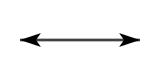 | Twofold rotation axis | 2 | — |
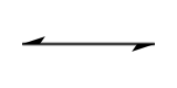 | Screw axis 2₁ | 2₁ |
Planes perpendicular to the drawing, symmetry lines
| Symbol | Element | Notation | Intrinsic translation |
|---|---|---|---|
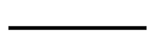 | Mirror plane; reflection line in the plane | m | — |
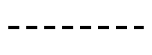 | “Axial” glide plane, glide in the drawing; glide line in the plane | a, b or c; g | of a translation along the line |
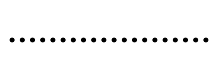 | “Axial” glide plane, glide towards the viewer | a, b or c | of a translation perpendicular to the drawing |
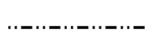 | “Double” glide plane (centred cells) | e | two glides: along the line and perpendicular to the drawing |
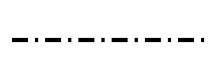 | “Diagonal” glide plane | n | one glide with two components, along the line and perpendicular to it |
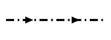 | “Diamond” glide plane (pair of planes, centred cells) | d | along the line and perpendicular to it; the arrow shows the direction in the drawing for which the perpendicular component is positive |
For a, b, c and n, the line style depends on the direction of the glide relative to the drawing, not on the letter: the same dotted line is a c plane in one description and an n plane in another (R3̄c in hexagonal or rhombohedral axes).
Planes parallel to the drawing
| Symbol | Element | Notation | Intrinsic translation |
|---|---|---|---|
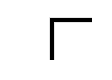 | Mirror plane | m | — |
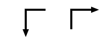 | “Axial” glide plane | a, b or c | of a translation in the direction of the arrow |
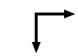 | “Double” glide plane (centred cells) | e | in the direction of either arrow |
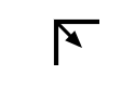 | “Diagonal” glide plane | n | in the direction of the arrow |
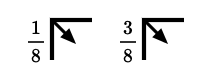 | “Diamond” glide plane (pair of planes, centred cells) | d | in the direction of the arrow, that is a quarter of a diagonal of the face-centred cell |
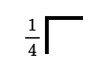 | A mirror plane at heights and | m | — |
These symbols are placed at the top left of the diagram, their branches along the cell edges. A fraction h denotes the pair of planes at heights h and h + ½; without a fraction, the planes are at heights 0 and ½.
In Laue
The Projection of the Tables looks at the cell from the side the chosen direction points to, like the diagrams: along c, a points down and b to the right, and a screw axis turns in the same sense as in the Tables. Leave the pointer on an element for a moment: a tooltip names it and gives its direction, its position () and its intrinsic translation; if several elements overlap, it lists them all.
Orbits, site symmetry and Wyckoff positions
Theory
The stabiliser of a point (its site symmetry) is finite, isomorphic to a subgroup of . A Wyckoff position is the set of points whose stabilisers are conjugate in . It is a union of orbits, parametrised by 0 to 3 free coordinates. Its multiplicity in the conventional cell is . The letters follow the order of the Tables, from the most symmetric (a) to the general position.
The choice of letter for a structure is defined only up to an automorphism: the Euclidean normaliser of permutes certain positions (4a and 4b of Fm-3m, for example). Two descriptions that differ in this way are the same structure.
The formulas
where is the number of lattice points in the conventional cell (1 for P, 2 for A, B, C and I, 3 for R in hexagonal axes, 4 for F).
In Laue
Wyckoff positions are computed by the engine from the operations: stabilisers, conjugation, affine varieties (points, lines, planes) modulo the lattice. Their letters and oriented symbols come from a reference table. The inspector of a site gives its position, its multiplicity and its oriented site-symmetry group (.3m, 4m.m). When dragged in the view, an atom snaps onto the special varieties it crosses, and Stay on constrains it to slide along its own. The coordinates remain exact.
Elements, composition and density
Theory
The content of the cell gives the formula, the number of formula units and the calculated density, the first check on a structure. Covalent radii give an expected bond length, the sum of the radii of the two atoms, which is useful for spotting bonds in an unknown structure.
The formulas
In Laue
The periodic table covers elements 1 to 103, with mass, configuration, Pauling electronegativity, covalent radius (Cordero et al., 2008) and common oxidation states (data from pymatgen). The formula follows electropositive order, and Hill order when the structure contains carbon. The bonds drawn join atoms whose distance approaches the sum of their covalent radii; two ions of the same sign are never bonded. Bonds that leave the cells (stubs) are hidden by default; unticking the Hide the bonds leaving the cells option shows them, for the full coordination.
Coordination polyhedra: the vertices are the neighbours bonded to the central atom (same criterion as the bonds drawn, up to atoms one cell beyond the box) and more electronegative than it; the polyhedron is their convex hull, its coplanar triangles merged into a single face (the squares of the fluorite cube). Default centres: the elements whose polyhedra have four to eight vertices; thus Ti and not Sr in SrTiO₃ (Sr has twelve O), V and not C in a carbide. The faces are depth-sorted together with the atoms and the bonds.
Structure formats
In Laue
The Structure menu reads and writes several formats.
- CIF (core CIF): the group is identified first from the set of operations
_space_group_symop_operation_xyz(or_symmetry_equiv_pos_as_xyz), compared with the 530 settings. Failing that, Laue reads the Hall symbol, then the HM symbol. Coordinates close to a fraction with a small denominator are snapped to it, and the atoms are put back on their special positions. - SHELX (
.ins,.res):LATTandSYMM, CELL, atoms. - POSCAR (VASP): all the atoms of the cell, without symmetry. Laue looks for the space group whose orbits reproduce the atoms, and keeps one atom per orbit. A primitive cell of a centred lattice is read as it is, in a smaller group.
- Write only: extended XYZ (ASE, Ovito), PDB (CRYST1) and CGD, the net read by Systre and the RCSR to name a topology.
Plane groups, orbifolds and two-colour groups
Theory
The 17 plane groups are the space groups of dimension 2: 5 Bravais lattices, 10 point classes. Conway and Thurston describe them by the topology of the quotient , the orbifold. Its notation lists the centres of rotation (digits), the mirrors (*), the mirror corners, the glides (×) and the handles (∘). The magic theorem gives the condition for an orbifold to be Euclidean: the costs add up to exactly 2.
The two-colour groups (black-and-white, or Shubnikov, groups) are the pairs with of index 2 in : the operations of swap the colours. There are 46 of them in the plane. Group–subgroup relations with the same cell (translationengleiche subgroups) connect the groups by loss of symmetry elements.
The formulas
Costs in orbifold notation: 2 for ∘, 1 for × and for *, for a centre of rotation of order off the mirrors, for a mirror corner of order .
In Laue
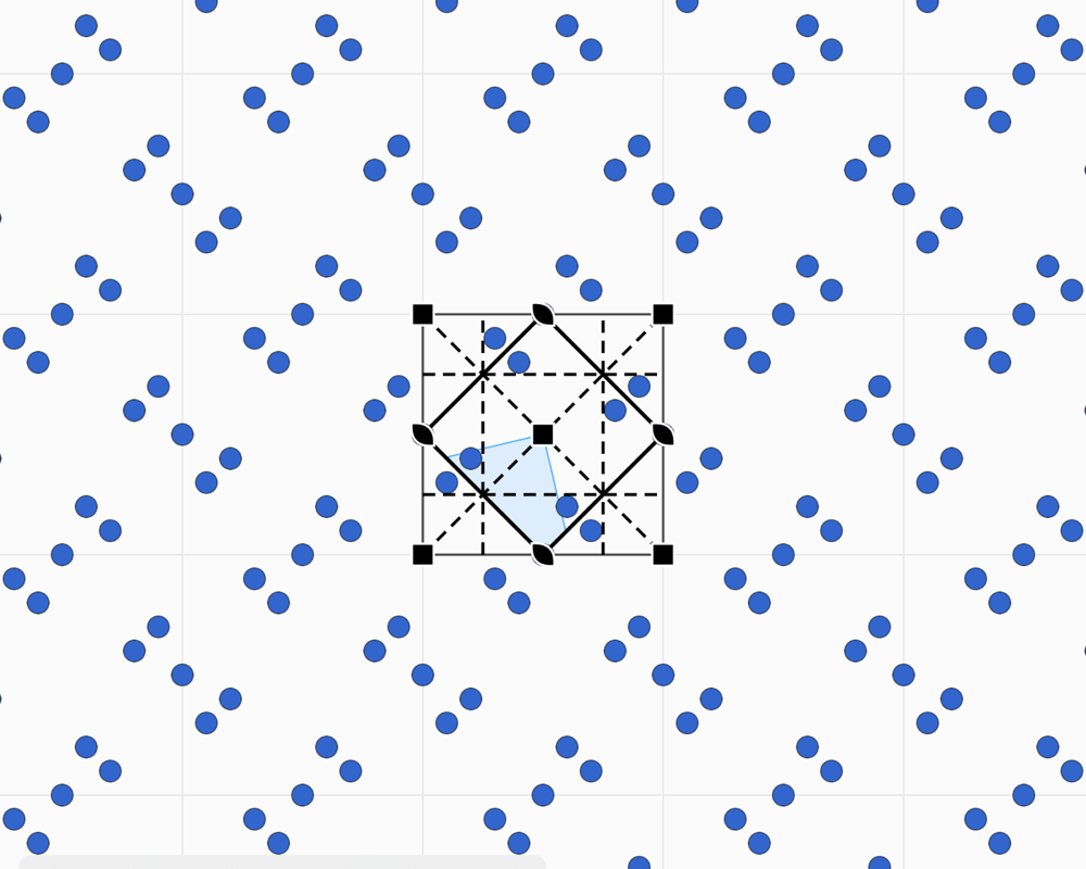
The plane workshop shows the groups by international symbol and orbifold. It shows the fundamental domain, the operations and the Wyckoff positions of the plane, as well as the subgroups and supergroups with the same cell. Two colours picks a subgroup of index 2; the operations that swap the colours are drawn in red. The Extent limits the drawing to a block of n × m cells from the origin cell (for a frieze, n cells), cut at the edge, for figures and exports. Placed motifs behave like the atoms of the Crystal workshop: they snap onto the special positions, and their multiplicity and site symmetry are checked.
Frieze groups
Theory
The seven frieze groups are the discrete subgroups of the isometries of the plane that leave a line invariant and whose translations form . They are written here with four-character symbols (p1, p1m1, p11m, p11g, p2, p2mm, p2mg), in orbifold notation (∞∞, *∞∞, ∞*, ∞×, 22∞, *22∞, 2*∞) and under Conway's names.
In Laue
The Tiling | Frieze | Rosette selector gives access to the friezes. The strip is drawn over the height b.
Rosette groups
Theory
The finite subgroups of are the cyclic groups and the dihedral groups (Leonardo's theorem). Their order is unrestricted. These are the point groups of the plane; the ten of them that are crystallographic (n = 1, 2, 3, 4, 6) are the classes of the plane groups.
In Laue
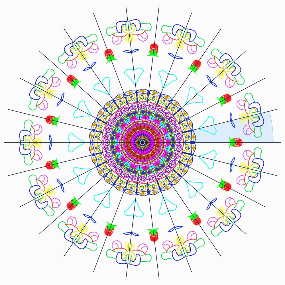
A rosette document carries the group “rosette Cn” or “rosette Dn”, with n from 1 to 24. It is shown in Schoenflies notation, in Hermann–Mauguin notation (8mm, 5m) and as an orbifold (8•, *8•). Positions are in Cartesian coordinates, with the radius of the figure equal to 1. The checks (copies, site symmetry, number of motifs) are those of the other workshops.
Kinematic theory of diffraction
Theory
In the Born approximation (single scattering), the scattered amplitude is the Fourier transform of the scattering density. For a crystal, this density is the convolution of the lattice with the content of the cell: the amplitude is non-zero only at the nodes of the reciprocal lattice, where it equals the structure factor. The atomic scattering factor , with , decreases with angle for X-rays (the electron cloud); it is constant for neutrons (coherent scattering length ). Isotropic thermal motion adds the Debye–Waller factor.
Systematic absences come from operations with a non-zero translation. For a centring, is multiplied by . For an operation , the reflections such that and are extinguished. These conditions, integral, zonal and serial, point to a set of compatible groups, not to a single group.
The measurement gives and loses the phases. Fourier synthesis requires them; the Patterson function, the autocorrelation of the density, does without them and shows the interatomic vectors. Direct methods and charge flipping recover the phases from the intensities alone; Laue does not implement them.
The formulas
In Laue
For plane patterns, Laue computes over all the scatterers of the cell, normalised to . Reflections extinguished by symmetry are marked with a ring, and the Laue class is given. The enlarged view (zoom up to ×64, with the visible region recomputed) exports as vector PDF and as CSV. Fourier synthesis rebuilds the motif with the true, zero or random phases, and the Patterson map shows the vectors between motifs.
Quasicrystals and model sets
Theory
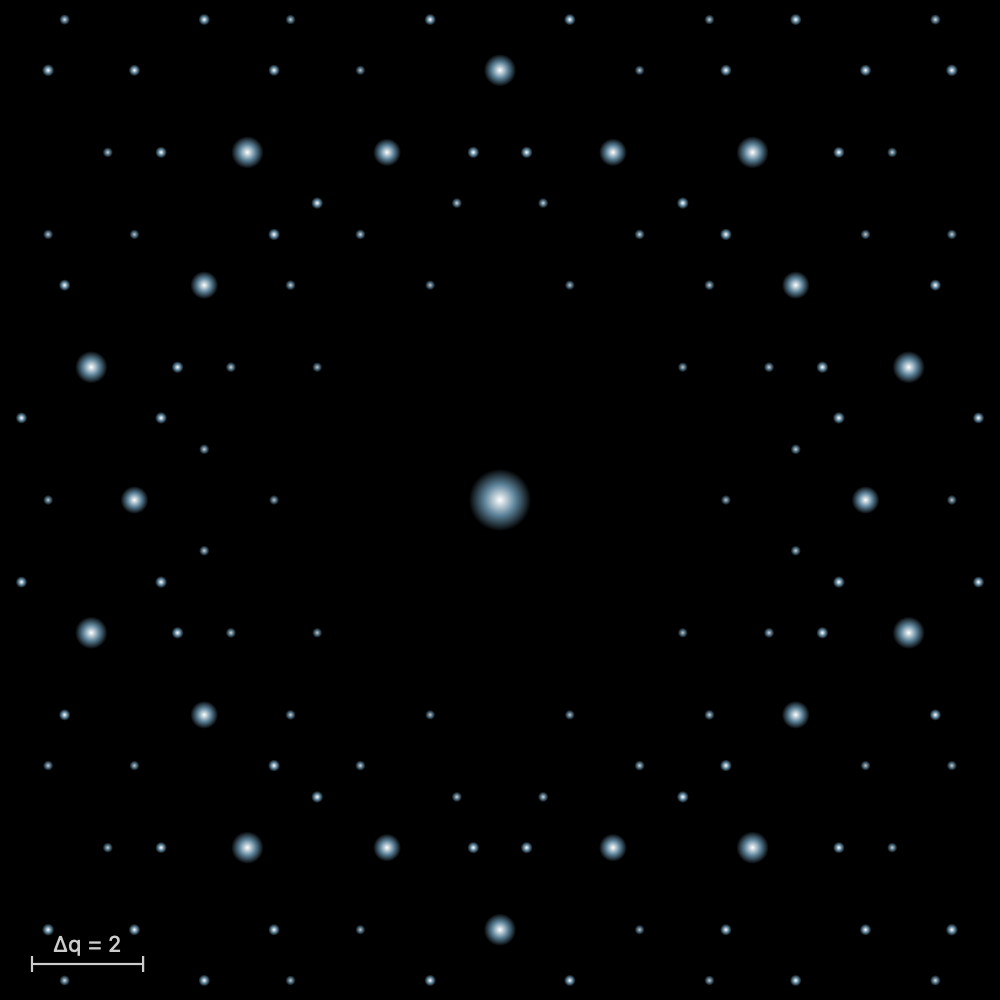
A model set (Meyer) is obtained by cut and projection. One starts from a lattice in irrational position, and keeps the points whose perpendicular projection falls inside a window . If the boundary of has measure zero, the diffraction spectrum is pure point. The peaks lie at the parallel projections of the dual lattice, with the amplitude of the Fourier transform of the window. The Fourier module has a rank higher than the dimension: 4 integer indices are needed to index the Penrose pattern.
Penrose comes from (pentagonal windows), Ammann–Beenker from (octagonal window). De Bruijn's multigrid method is dual to the cut: one tile per crossing of two families of lines. A uniform shift of the window (the phason degree of freedom) produces a locally indistinguishable tiling, up to tile flips. The inflation factor is for Penrose and for Ammann–Beenker.
The visible points of a lattice, with coprime coordinates, form a weak model set. It is not a Delone set (it has arbitrarily large holes), yet its diffraction is pure point (Baake, Moody and Pleasants, 2000).
The formulas
-free points of (: the visible points), density and Bragg intensities at the points whose denominator is -th power free:
In Laue
The workshop builds the three tilings by the multigrid method (5, 4 and 6 families of lines), and Penrose also by inflation. The Phason sliders shift the grids, and Perpendicular space shows the image of each vertex in . Diffraction is computed on the vertices: Bragg peaks, or an intensity map on a logarithmic scale. The decorations (Penrose arcs, girih strapwork, de Bruijn ribbons) and the tile designer are ornament; they do not change the diffraction of the vertices.
Laue method
Theory and model
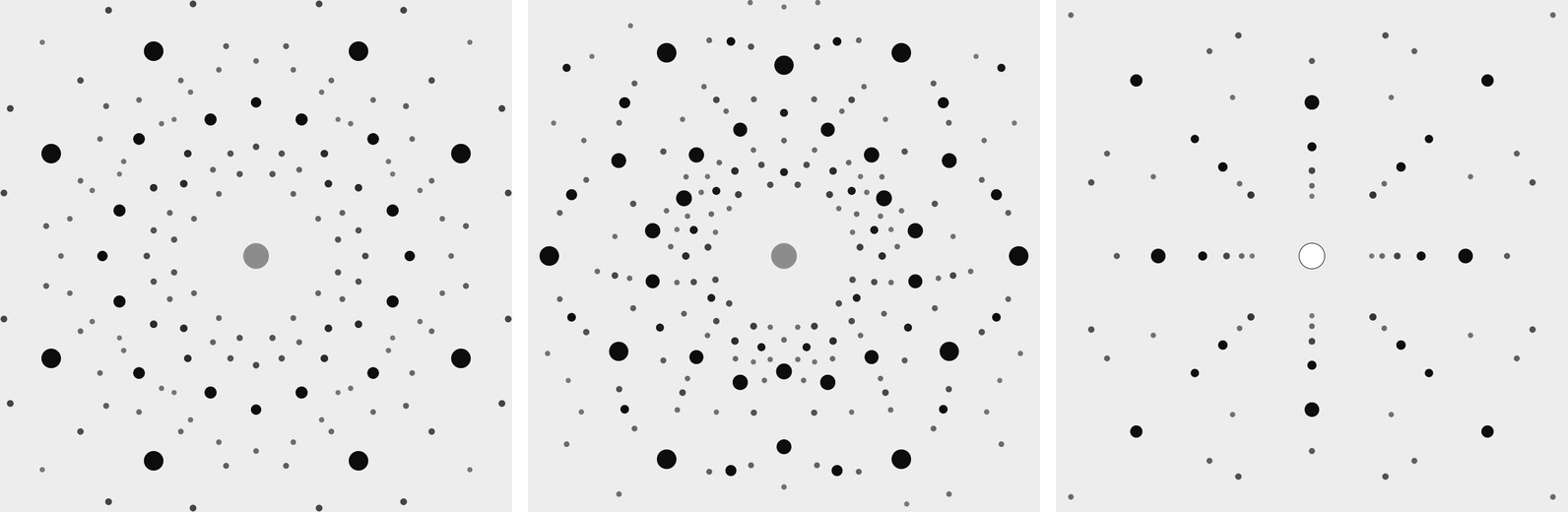
A stationary single crystal is illuminated by white radiation, from to . In the Ewald construction, all the spheres of radius between these bounds are present at once. Each reciprocal-lattice node lying between the smallest and the largest sphere diffracts the wavelength whose sphere passes through it. The diffracted direction depends only on the direction of : the harmonics are superimposed in one spot, with . The planes of a zone with axis diffract on a cone with axis . On a flat film, this cone traces an ellipse in transmission and a hyperbola in back-reflection.
Friedel's law makes the pattern centrosymmetric in intensity, in the absence of anomalous scattering. Its symmetry is the subgroup of the Laue class that fixes the beam direction: 4mm along [001] for , 3m along c for . The method thus identifies one of the eleven Laue classes and gives the orientation, but not absolute intensities: each spot mixes several wavelengths and several harmonics.
Laue's model assumes a flat spectrum within the band, an unpolarized beam, and no absorption, extinction or mosaicity: the spots are points. The intensity of a spot is the sum, over its harmonics present in the band, of multiplied by the polarization factor and the Lorentz factor of the Laue method, . Intensities are normalized to the strongest spot.
The inverse problem gives the orientation. A spot at on a film at the distance fixes the direction of the diffracted ray. The normal of the reflecting planes is parallel to , since . Its projections on , and are proportional to , , , because . Only the direction of is accessible: , and hence , remain unknown. To index, the angles between normals, computed with the reciprocal metric tensor, are compared with those of a model. Two indexed spots then suffice to fix the orientation matrix (Busing and Levy, 1967). In back-reflection, the angles are traditionally read on the Greninger chart.
The formulas
In Laue
The beam points along the view, from 0.25 to 2.5 Å. Once per structure, Laue computes all the planes with primitive indices , with for each harmonic such that . The scattering factors are those of Waasmaier and Kirfel, with = 0.5 Ų. A reflection extinguished by symmetry counts as zero. Rotating the view recomputes only the geometry. The film is flat, 100 mm square, at = 40 mm; spots weaker than 10−3 of the strongest are omitted. The tests check the 4mm symmetry of NaCl along [001] in both geometries, the 3m symmetry (not 6mm) of quartz along c, Bragg's law for each harmonic and the position . Enlarged, the pattern sets the radiation (X-rays, λmin = 12.398/kV Å after Duane–Hunt; or neutrons, with the coherent scattering lengths and no polarisation factor), λmax and D; pointing at a spot gives hkl, its harmonics and their λ, 2θ, d and the intensity, and the table of spots exports as CSV. The film frame is that of the view: looking along [u v w], up is c (or b along c) and right is up × (−n̂). The tutor asks three questions on this model: the symmetry of the pattern along an axis (the subgroup of the Laue class that fixes the beam), the deviation 2θ of a spot, and the indices of the spot at (x, y).
Calculated powder pattern
Theory and model
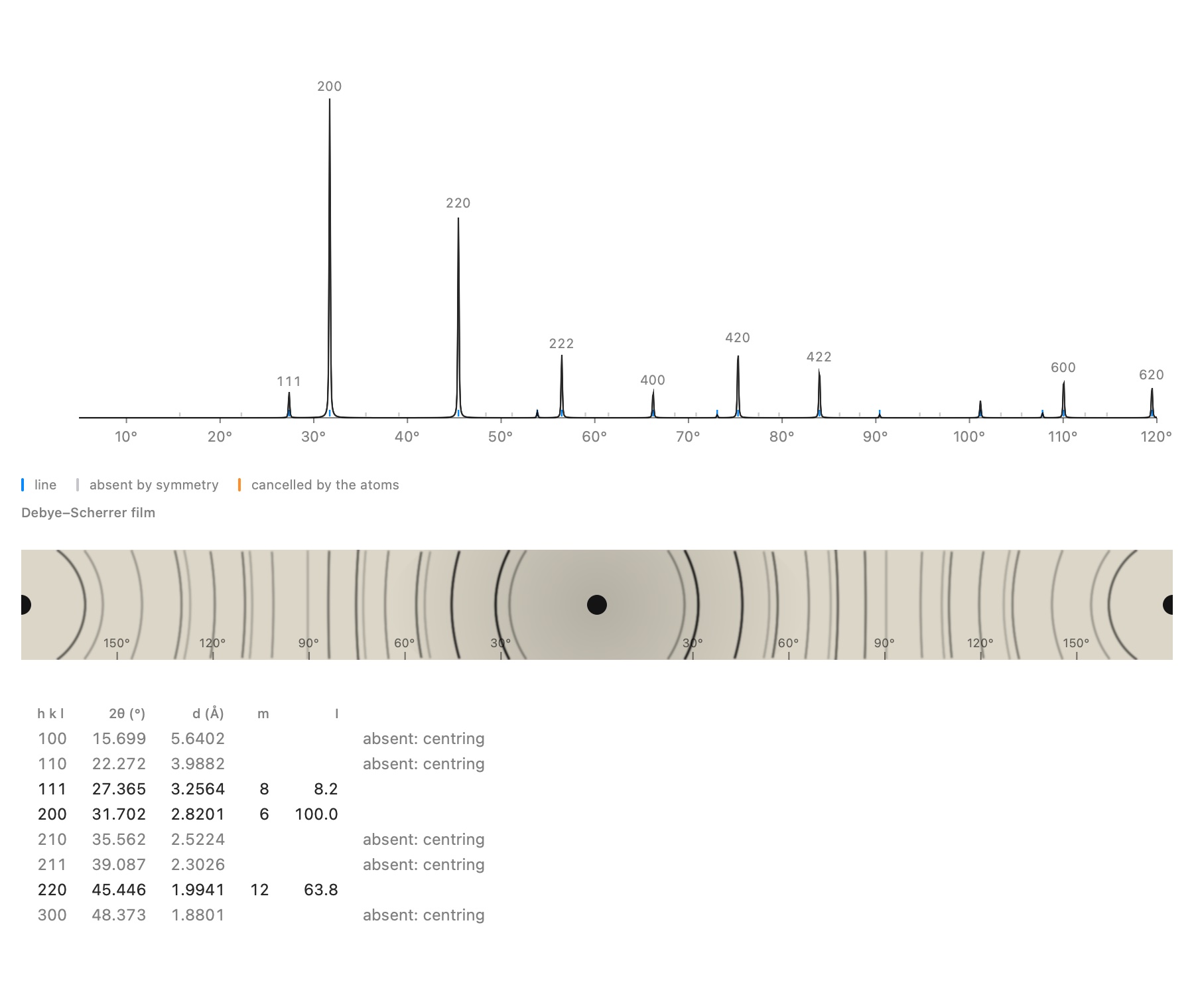
For an ideal powder (random orientations, crystallites with no extinction and no differential absorption), the integrated intensity of a line is the sum of the of the reflections with the same . It is multiplied by the Lorentz-polarisation factor for an unpolarised beam. Laue applies no monochromator factor and models neither preferred orientation, nor absorption, nor extinction. A line gathers the reflections with the same , whether equivalent by symmetry or coincident by accident; its multiplicity is the number of reflections present. The Kα₂ doublet is added with an intensity ratio of 0.5.
The formulas
In Laue
The pattern below the view is recomputed at every change. The enlarged viewer sets the radiation (Kα₁ of Cu, Co, Mo, Cr and Ag anodes, a free wavelength, or neutrons), the wavelength, Kα₂, an overall , the width and 2θmax. For each zero reflection, the table of lines states whether it is extinguished by symmetry (centring, screw axis, glide plane) or cancelled accidentally by the atomic positions (222 of diamond). Identical points sets with no fall-off: only the geometric factor of the lattice and the positions remains.
Profile fitting on a measurement
Model
Laue fits the profile part of a Rietveld refinement. The integrated intensities are those of the document's structure: atomic positions and values are not refined. The free parameters are the scale, the zero, the sample displacement (Bragg–Brentano geometry), the background, the widths, the mixing, the asymmetry and the cell. The minimisation is of Levenberg–Marquardt type, in two passes, with weights ( when no standard deviation is supplied).
The formulas
with , , the zero and the sample displacement.
Bérar–Baldinozzi asymmetry (1993), with , , :
Chebyshev background over the measured range, :
Agreement factors:
In Laue
Formats read: .xy, .xye, .dat and CSV (2θ, I, σ), powder CIF (_pd_meas_*) and GSAS (STD, ESD). Tick the parameters to release and bound the 2θ range, then Refine runs the fit in the background. The result gives , , and the cell; Apply the cell writes it into the document. Validation: a real measurement of NIST SRM 660 (LaB₆, Cu Kα₁ + Kα₂, GSAS-II tutorials), fitted from 40 to 125°; the certified cell is recovered to within 3 × 10⁻⁴ Å.
Peak search and indexing
Theory
Indexing looks for a positive definite quadratic form that reproduces the observed with integer indices. Systems with one or two parameters are handled through the allowed forms: sums of three squares other than for cubic, sums of two squares for tetragonal, Löschian numbers for hexagonal. Quality is measured by (de Wolff, 1968).
The formulas
In Laue
The peaks are the maxima of the smoothed intensity, at least 6 σ above the background. The first 20 are indexed in the cubic, tetragonal, hexagonal and orthorhombic systems (no monoclinic or triclinic search). The tolerance is 0.03° on each 2θ, widened by 0.15° during the search to allow for a zero shift. Cell edges are limited to 20 Å and the volume to 2000 ų. A less symmetric system is explored only if the more symmetric ones give no cell with . Solutions are ranked by , with those that index every line but at most one placed first. For a chosen cell, the families of space groups compatible with the absences are offered, from the most restrictive to the least.
Band structures and absorption
Brillouin zone and paths
The Brillouin zone is the Wigner–Seitz cell of the reciprocal lattice, bounded by the perpendicular bisector planes of the shortest reciprocal vectors. Laue follows Setyawan and Curtarolo (2010): for each lattice type, and for its variants according to the ratios of the parameters (BCT1 and 2, ORCF1 to 3, RHL1 and 2…), they fix the high-symmetry points, their names and the usual path. The lines bear their usual names (Δ, Λ, Σ, Z, Q, S…). For monoclinic and triclinic lattices the path is simplified: Γ and the midpoints of the three shortest reciprocal vectors.
The three models
- Empty lattice. : plane waves folded back into the zone.
- Empirical pseudopotential of Cohen and Bergstresser (1966), for fourteen semiconductors with the diamond or zinc-blende structure. The symmetric and antisymmetric form factors are taken at . The plane-wave basis, , is chosen for each k, and the diagonalisation is done by LAPACK. Si: indirect gap of 0.82 eV (1.12 eV measured), conduction minimum at 85% of Γ–X. GaAs: direct gap of 1.43 eV (1.42 eV).
- Virtual crystal (Nordheim, 1931), for alloys whose compounds are in the table: the form factors V_S and V_A are the average of those of the compounds, weighted by the products of the fractions on the two sites (In₁₋ₓGaₓAs: (1 − x) InAs + x GaAs; a quaternary, its four binaries), and likewise the spin–orbit μ. The cell follows Vegard's law between the lattice parameters measured at room temperature (Madelung, 2004). Checks: the switch from the Δ valley to the L valley in Si₁₋ₓGeₓ near x = 0.93 (measured 0.85; Braunstein, Moore and Herman, 1958); from Γ to X in GaAs₁₋ₓPₓ near x = 0.36 (measured 0.45); In₀.₅₃Ga₀.₄₇As, 0.91 eV against 0.75 eV measured. Limits: disorder is ignored, hence too weak a gap bowing (the “special quasirandom” supercells of Zunger et al., 1990, give it); a single set of phonons; AlAs is missing from the table, so AlₓGa₁₋ₓAs has only Vegard's law and tight binding.
- Tight binding with Harrison's universal parameters (1999). Each atom carries its s and p orbitals, plus d orbitals for transition metals, at Mann's atomic term values. The hopping integrals are between s and p, with and for d, distributed by the Slater–Koster table (1954). The nearest neighbours count in full, then the shells up to twice that distance, damped as with . The number of valence electrons follows the column of the periodic table. Filling on a 16³ grid distinguishes metal, semimetal (bands within 0.1 eV of each other) and insulator. No overlap matrix, no Madelung shift, no spin: the gaps of ionic crystals and oxides come out too wide (NaCl: 9.0 eV for 8.5; SrTiO₃: 5.3 eV for 3.2).
Density of states and optics
The density of states is computed on a 16³ grid reduced by the point group and time reversal, and smoothed with Gaussians. The imaginary part of the dielectric function comes from the momentum matrix elements between valence and conduction bands; in tight binding these are the Peierls ones, . It is integrated by the tetrahedron method (Blöchl, Jepsen and Andersen, 1994), with local refinement near the edge. The grid is refined from 12³ to 28³ until convergence: ε₁(0) within 1%, ε₂ within 3% of its maximum, the edge within 0.03 eV. ε₁ follows by Kramers–Kronig, then n, κ, α and R. The Tauc plot fits a straight line to for a direct gap and to for an indirect gap, between the edge − 0.05 and the edge + 0.4 eV. The scissors raise the conduction bands by an amount Δ, and the matrix elements are corrected as proposed by Levine and Allan (1989). Silicon: ε₁(0) = 11.2 (11.7 measured).
The formulas
In Gaussian units, with the factor 2 for spin:
The scissors (Levine and Allan):
Spin–orbit coupling
The spin of the electron couples to its orbital moment: at Γ, the top of the valence band, of p character, splits into Γ₈ (j = 3/2, four states) and Γ₇ (j = 1/2, two states), lower by Δ₀, from 0.044 eV in Si to 0.95 eV in CdTe; at L, the splitting Δ₁ is about two thirds of Δ₀. The basis becomes that of spinors: each band now holds only one electron, and there are twice as many bands. In the pseudopotential, the Weisz term, in the form of Chelikowsky and Cohen (1976), has a strength μ fitted to the measured Δ₀; it predicts Δ₁ with no further adjustment (GaAs 0.21 eV for 0.22 measured, InSb 0.50 for 0.50). In tight binding, each atom receives λ L·S on its p orbitals, λ being proportional to the constant ζ_np of the free atom, taken from its measured fine structure (NIST database); a single factor, 1.54, fitted on thirteen semiconductors, gives Δ₀ to within 15%.
The formulas
Fermi surface
For a metal in tight binding (the Fermi level fixed by counting the electrons on the 16³ grid) or for free electrons (, n being the s and p valence electrons per volume: 1 for Cu, Ag, Au and the alkali metals, 2 for Mg, Zn and iron, 3 for Al…), the bands are computed on a cubic grid of 31³ points covering the zone. Each small cube is cut into six tetrahedra in which E is interpolated linearly: the surface E = E_F is a triangle or a quadrilateral there (marching tetrahedra, with no ambiguous case). Each crossing point is refined on the band itself by two steps of false position; the triangles are clipped at the faces of the zone (Sutherland–Hodgman) and oriented along the gradient of E, towards the empty states. The occupied part of each band is counted on a 20³ grid of the primitive reciprocal cell, whose volume is exactly that of the zone. Checks: the free sphere of copper has the radius k_F = 1.36 Å⁻¹ and the area 4πk_F²; its occupied bands hold one electron, those of aluminium three, those of copper in tight binding eleven, to within 1%; in tight binding, the surface of copper touches the eight {111} faces, at the L points.
In Laue
Band structure (Properties tab) places a small diagram beside the view. The enlarged viewer shows the zone in relief, the bands with the gap and its nature, the density of states and, for a semiconductor or an insulator, the Absorption tab (ε₁ and ε₂, n and κ, α, R, Tauc). The method can be chosen: pseudopotential when the crystal is in the table, tight binding for any crystal that has atoms, empty lattice always. The Spin–orbit coupling switch adds spin to the first two. Measured gap sets the scissors to the value given by Madelung (2004). The bands, the density of states and the spectrum export as CSV, the graphs as PNG or PDF. The same computations run from the command line (laue bands, laue optics), and their outputs serve as the reference for the Windows port.
The scissors move the spectrum rigidly, ε₂(E) → ε₂(E − Δ), as Levine and Allan's correction implies: the transitions are binned once, without scissors, and each position of the slider only shifts them and redoes the Kramers–Kronig integral. In tight binding, every empty band (up to 16) enters the spectrum, computed up to the edge + 6 eV at least (10 eV otherwise); the refinement around the edge is reduced when its minima cover more than 5 % of the zone (flat bands, such as calcite's), and left out beyond a quarter. The computation shows the grid it is on and can be stopped.
The spectrum is a tensor: each transition stores Re(q_a q_b*) as six components, then averaged over the rotations of the point group (J̄ = Σ_R R J Rᵀ / |G|, exact with the tetrahedra); the principal axes are those of ε₁(0) − 1 ∝ Σ J/E³, and Polarisation projects onto one of them before the scissors and Kramers–Kronig, with no new computation. The indices at 589 nm from Point dipoles (Tessman, Kahn and Shockley polarisabilities, local field by Ewald sums) and from Bands, with the gap correction were compared with measurements on thirteen crystals: point dipoles within 4 % for the ionic insulators with a gap of 5 eV or more, the bands 2 to 7 % low for the semiconductors and about 20 % low for rutile and SrTiO₃ (minimal basis, no local field). The rule drawn from this marks the Recommended model: point dipoles when every ion is tabulated and the gap reaches 5 eV, the bands otherwise; it picks the closer one on all thirteen. The bands give the sign of nₑ − nₒ right in the five uniaxial crystals, point dipoles in two. Intra-atomic dipole terms (Pedersen et al. 2001) were tried: with Harrison's universal parameters they move every crystal away from the measurement, and stay off. From the command line: laue indices.
Dispersion: each measured curve is the published formula (Sellmeier and related forms of the refractiveindex.info database, coefficients unchanged), which gives the table's index back to 0.002 at 589.3 nm. V_d = (n_d − 1)/(n_F − n_C) at the 587.6, 486.1 and 656.3 nm lines. Point dipoles give only one index, so their dispersion is a single oscillator of Wemple and DiDomenico, n² − 1 = E_d E₀/(E₀² − E²), through that index at the E₀ fitted to the bands' curve; the Sellmeier shown is the same thing rewritten (B = E_d/E₀, C = (hc/E₀)²). On thirteen crystals, V_d is within 20 % for 11 rays out of 14; CsCl, calcite's ordinary ray and ZnS are 30–41 % off. The oscillator fitted to the measurement and to the bands tells what the bands lack: E₀ within 8 % for 11 rays out of 16, but a strength E_d 37 to 61 % too weak in the ionic crystals and the titanium oxides — this is what leaves rutile and SrTiO₃ 20 % below the measurement. Wemple's empirical rule E_d = β N_c Z_a N_e, tried as a third model, mends rutile's ordinary ray but overshoots SrTiO₃ by 18 % and reverses the sign of the birefringence in three uniaxial crystals: it is not offered. From the command line: laue dispersion.
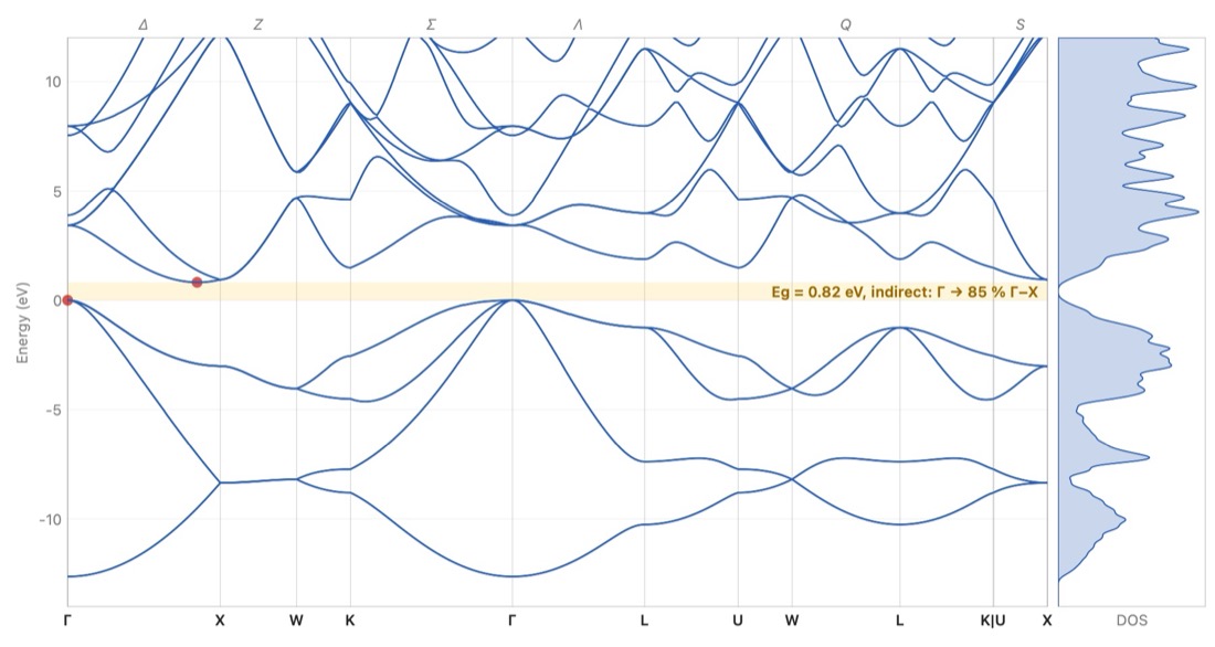
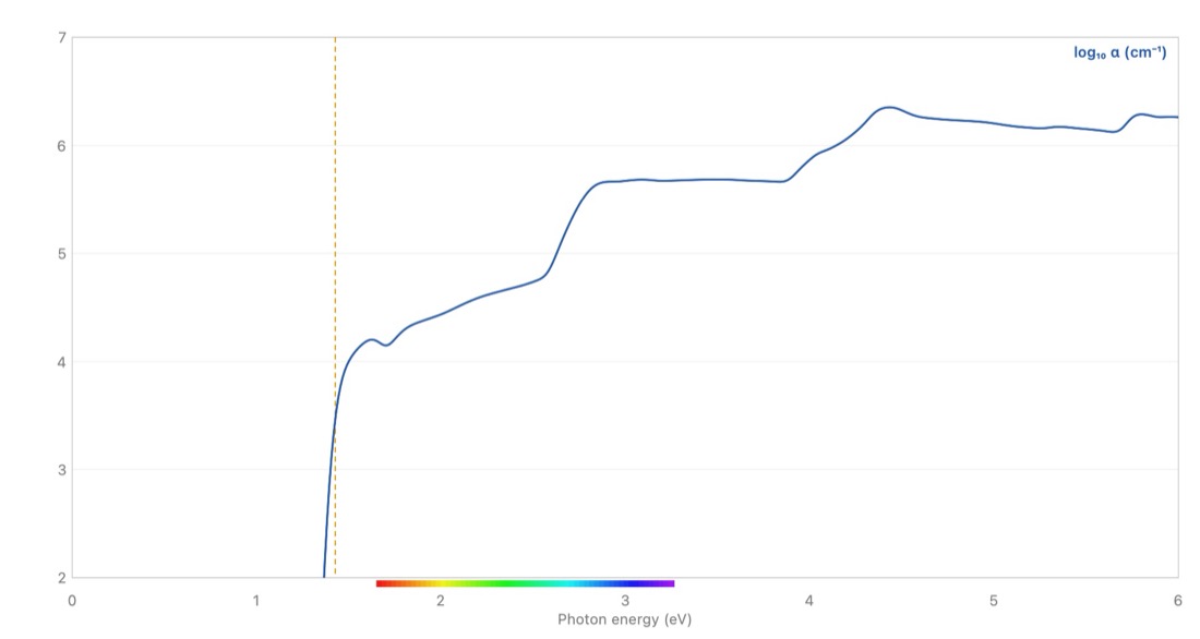
The viewer can be resized, and each of its graphs can be enlarged: dragging a frame with ⌥ zooms into it (a flat frame zooms along one axis only), dragging without ⌥ or scrolling with two fingers moves the enlarged graph, the mouse wheel zooms under the pointer and pinching around the centre, ⌥ with scrolling or the + and − buttons in the corner zoom vertically only, and a double-click or the button in the corner returns to the whole graph; on iPad, a finger moves and pinching zooms. The density of states follows the energy axis of the bands.
Phonons: spring model
Model
Laue computes the vibrations in the harmonic approximation of Born and von Kármán. The energy is a sum of terms , invariant under translation: the acoustic sum rule is therefore satisfied by construction. The form is Keating's (1966): a stretching spring α on each bond and a bending spring β on each angle between two bonds of the same atom.
- Keating, Martin's parameters (1970), fitted to the elastic constants, for Si, Ge, GaP, GaAs, GaSb, AlAs, AlSb, InP, InAs and InSb (four neighbours). Si: 16.5 THz at Γ (15.5 measured); at X, LA = LO 12.9 (12.3) and TO 14.5 (13.9). The TA branches come out too high at X and L (7.7 THz for 4.5), a known shortcoming of the model.
- Universal springs for any other crystal, on the first shell of neighbours (up to 1.2 times the shortest distance between two metal atoms): according to the character of the bond. Covalent: = 48.5 N/m, = 2.35 Å, = 4, β = 0.28 α. Metallic: calibrated on the maximum of copper at X (7.25 THz), with no bending; two cations of an ionic crystal are not bonded.
- Rigid ions (Kellermann, 1940) when a bond is ionic (electronegativities at least 1.7 apart): formal charges (the anion at its usual oxidation state, the cations at their highest, brought back to neutrality), Coulomb forces summed by Ewald's method, and a Born–Mayer repulsion between nearest neighbours, radial and tangential, with λ set by the equilibrium of the crystal under a uniform dilation and ρ = 0.3036 Å calibrated on the TO of NaCl at Γ (4.92 THz). The term is screened by ε∞ (measured for common crystals, 2.5 otherwise); at Γ, its limit follows the direction from which the path arrives. NaCl: LO 7.4 THz (7.9); CaF₂: TO 7.6 (7.7), LO 12.9 (14.0); CsCl: TO 2.9 (3.0). Cubic SrTiO₃ is unstable at R: the rotation of the octahedra that makes it tetragonal below 105 K. Formal charges overestimate the highest modes of oxides.
- Polar semiconductors of Martin (GaAs, InP…): the dipole term alone, with the Born effective charge and ε∞ (GaAs: 2.07 and 10.9; LO − TO = 0.56 THz for 0.53).
- Layers (an atom whose bonds all lie in one plane): a term against bending out of the plane, C = 0.586 α, and springs of 0.911 N/m to the nearest atoms of the neighbouring layers, calibrated on graphite (out-of-plane B2g, 26.1 THz; E2g shear, 1.26 THz).
The formulas
Keating, with Martin's convention (, ), and the dynamical matrix:
In Laue
The Phonons tab of the viewer draws the 3N branches along the path of Setyawan and Curtarolo and the vibrational density of states (16³ grid reduced by symmetry, three modes per atom), in THz, cm⁻¹ or meV. For the universal springs and the rigid ions, a slider multiplies all the short-range stiffnesses. An unstable mode is drawn below zero. laue phonons also gives the charges, ε∞, λ and the LO limit at Γ along [100]. Branches and density export as CSV; laue phonons gives the frequencies at the points of the zone.
Light: infrared, Raman and indices
Activities at Γ
The modes at Γ are the eigenvectors of the dynamical matrix at q = 0 (without the non-analytic term: the TO frequencies). Modes degenerate to within 10⁻⁶ form subspaces W. Their activity comes from the characters, without a group table: the operations of the space group act on the displacements through Γ(g) (Cartesian rotation and permutation of the atoms of the primitive cell), and one counts the multiplicity of the vector representation (dipole: infrared) and of its symmetric square (polarisability: Raman). Validation: Si F2g Raman only, NaCl F1u infrared only, CaF₂ one mode of each, GaAs F2 both, corundum 7 Raman and 6 infrared modes (Porto and Krishnan, 1967), mutual exclusion in every centrosymmetric crystal.
Infrared
The oscillator strength of a mode comes from its effective charge , with the Born charges: formal for the rigid ions, tabulated for Martin's semiconductors. The reflectivity is computed at normal incidence, with a damping γ = 0.02 ω_TO. NaCl: ε(0) = 5.3 (5.9 measured), reststrahlen band from 164 to 246 cm⁻¹ (164 to 264). Corundum: ε(0) = 9.8 perpendicular to c and 11.3 parallel (9.4 and 11.6 measured).
The formulas
Indices in the visible: point dipoles
Each ion carries an electronic polarisability α (Tessman, Kahn and Shockley, 1953; Pauling, 1927; that of O²⁻, 1.30 ų, is calibrated on the ordinary index of calcite). The field acting on an ion is the macroscopic field plus that of all the other dipoles, summed by Ewald's method without its q = 0 term (which contains the Lorentz field); one solves , then . NaCl: 1.542 (1.544); CaF₂: 1.404 (1.434); calcite: nₒ 1.658, nₑ 1.54 (1.486), two thirds of the negative birefringence recovered; corundum 1.72 (1.76); quartz 1.51 (1.55). The model fails for titanates (1.7 instead of 2.4 to 2.9): their bonds are too covalent for point dipoles. The optical class follows from the crystal system.
Colour centres
A colour centre does not change the symmetry with which Laue computes: it only adds absorption bands, Gaussian in energy. Cr³⁺ (d³) on an octahedral site follows the Tanabe–Sugano diagram, with Dq and B measured for ruby (1810 and 650 cm⁻¹) and emerald (1610 and 780 cm⁻¹), elsewhere Dq ∝ R⁻⁵ scaled from ruby; widths 0.33 eV (⁴T₂) and 0.60 eV (⁴T₁). Ruby: 2.24 and 3.07 eV (2.23 and 3.05 measured). F centre: the law of Mollwo and Ivey, d being the distance to the nearest cation; NaCl 2.61 eV (2.65), KCl 2.15 (2.3), width 0.18 E. Tabulated bands (Burns, 1993; Nassau, 2001): Fe²⁺–Ti⁴⁺ of sapphire, Fe²⁺ of aquamarine, NV⁻ of diamond, Fe³⁺. The varieties of quartz (Rossman, 1994): amethyst, [FeO₄]⁰ centre at 545 and 357 nm; smoky quartz, [AlO₄]⁰ centre near 450 and 620 nm with an absorption rising towards the ultraviolet; citrine, O → Fe³⁺ charge transfer near 375 nm, whose tail takes the blue; rose quartz, a broad band near 500 nm. Each band carries its wavelength in the menu, beside the levels in the bands and as a marker on the absorption curve. The colour: transmission , CIE 1931 colour-matching functions in the analytic approximation of Wyman, Sloan and Shirley (2013), a black body at 6504 K for D65, sRGB balanced on white.
The formulas
The other transition-metal ions follow the same diagrams in closed form, with Dq and B fitted to measured bands: those of the hydrated ion [M(H₂O)₆]ⁿ⁺ (Lever, 1984) for want of anything better, those in corundum where they have been measured (McClure, 1962). d¹ and d⁶ (Ti³⁺, Fe²⁺) and d⁹ (Cu²⁺) have only one spin-allowed band, at 10 Dq, which the Jahn–Teller effect splits in two: Ti³⁺ in corundum, 18,450 and 20,300 cm⁻¹ (542 and 493 nm). The ground state of d² (V³⁺) is ³T₁(F), mixed with ³T₁(P): in corundum (Dq 1870, B 620 cm⁻¹), 17,400 and 25,400 cm⁻¹, against 17,400 and 25,200 measured. On a site with four neighbours, the field is 4/9 of that of the octahedron, and the ion with n electrons follows the octahedral diagram for 10 − n: Co²⁺ (d⁷) in a tetrahedron behaves as d³, and its ν₃ near 17,200 cm⁻¹ (582 nm) gives cobalt blue. Brought back into an octahedron (Dq × 9/4), the same set of parameters predicts the bands of [Co(H₂O)₆]²⁺: 8000 and 19,000 cm⁻¹, against 8100 and 19,400 measured. The d⁵ ions (Mn²⁺, Fe³⁺) have no spin-allowed band; they are not among the ions.
Dichroism. In a uniaxial crystal, the absorption depends on the polarisation. For ruby, Laue takes the bands measured by Cronemeyer (1966): E ⊥ c at 558 and 412 nm, E ∥ c at 543 and 398 nm, with their cross sections (22.8 and 22.5 × 10⁻²⁰ cm² against 7.2 and 38.1). For blue sapphire, the Fe²⁺–Ti⁴⁺ band moves from 580 nm (E ⊥ c) to 700 nm (E ∥ c), about 250 nm wide (Dubinsky et al., 2020); the source does not give a figure for its E ∥ c cross section, which is taken as equal. The optical density that is set remains that of unpolarised light, the average of the two: ruby comes out purplish red for E ⊥ c and orangy red for E ∥ c, sapphire violetish blue and blue-green, as in the dichroscope.
Concentration. With a cross section σ measured at the E ⊥ c peak (corundum: Cr³⁺ 1.62 × 10⁻¹⁹ cm² at 560 nm, V³⁺ 1.0 × 10⁻¹⁹ cm² at 580 nm, Fe²⁺–Ti⁴⁺ 1.94 × 10⁻¹⁸ cm² at 580 nm; Dubinsky et al., 2020), the optical density over the reference thickness d = 5 mm gives the density n of centres, referred to the number of atoms per cm³ of the crystal. A ruby of optical density 2 thus contains about 800 ppma of chromium. For Fe²⁺–Ti⁴⁺, σ is that of the pairs per iron atom, at about 4700 ppma of iron: it decreases as the iron becomes scarcer, and the concentration is only an order of magnitude.
The formulas
In Laue
The Infrared and Raman tab of the viewer gives the table of modes, the reflectivity (E ⊥ c and E ‖ c for a uniaxial crystal), the optical class, the indices, ε∞ and ε(0). From the command line, laue infrared. Limits: calcite remains unstable at the zone boundary and beryl does not hold together with these rigid ions; the activity of their modes at Γ remains correct.
The colour centres of the document also appear in the band viewer. Their levels, flat because a centre is localised, are drawn in the gap with one arrow per transition, and their peaks are added to the density of states, enlarged: the real weight of a centre is its concentration, a few parts per million. The spacing between the levels is the energy of the transitions; their position in the gap is a convention, not a calculation. The 2p level of an F centre lies 0.15 eV below the conduction bands (the thermal depth given by Mott and Gurney for KCl), and 1s lies below it; for Cr³⁺ and the tabulated bands, the ground level is where the slider puts it, mid-gap by default. The states of Cr³⁺ (⁴A₂, ⁴T₂, ⁴T₁) are many-electron terms, drawn as levels. For Cr³⁺, the ²E level is drawn too, at the measured energy of the R₁ line (694.3 nm in ruby, 683.0 nm in emerald, that of ruby elsewhere): pumping into ⁴T₂ and ⁴T₁ relaxes without light to ²E (wavy arrow), a metastable state of about 3 ms where the ions accumulate, from which the R line to ⁴A₂ starts (red arrow), the line of Maiman's ruby laser (1960). The transition ⁴A₂ → ²E changes the spin: a thousand times weaker than the ⁴T bands, it does not enter the absorption. In the Absorption tab, their bands are added below the edge: with d = 5 mm, the thickness of a cut stone, then and ε₂ increased by 2nκ; ε₁ is not corrected, since the share of the centres in ε₂ is of the order of 10⁻⁵. The α scale then goes down to 0.1 cm⁻¹.
Zeeman effect of ruby's R lines, field B along c. The ground ⁴A₂ (S = 3/2) splits as , g∥ = 1.9817 and 2D = −11.493 GHz, the ±3/2 doublet lowest (Sewani et al., 2020); the levels Ē (line R₁) and 2Ā (R₂, 29 cm⁻¹ higher) each split in two, ±½ g μ_B B, with |g∥(Ē)| = 2.44 and g∥(2Ā) = 1.46 (Gen et al., 2020). The allowed components and their relative strengths follow Sugano and Tanabe (1958), in the table of Gen et al.; σ lines are about seven times stronger than π, their experimental estimate. Shifts are in cm⁻¹ from each line, μ_B = 0.4669 cm⁻¹/T; at zero field each line is already double, by 0.38 cm⁻¹ (2D).
Temperature: lattice thermodynamics
Harmonic approximation: the modes of the Phonons section (same springs, stiffness factor 1) on a q grid over the whole Brillouin zone, centred on Γ to keep the symmetry of the crystal (12³ q up to 4 primitive atoms, 8³ up to 16, 6³ beyond), Γ itself excluded: its acoustic modes have no frequency, and there the optical modes of an ionic crystal depend on the direction of approach. Each mode is a quantum oscillator. Per atom: , , , x = hν/k_BT, sums weighted by 1/N_q and divided by the number of atoms. Unstable modes (imaginary frequency) are discarded and counted.
Debye temperature: at T, that of the Debye model giving the same C_v, , inverted by bisection; at high temperature, (second moment). Displacements: , with the eigenvectors of the mass-weighted dynamical matrix. For accuracy at low frequencies, coth y = 1/y + (coth y − 1/y): the first term, in T/ω², is summed exactly, the second, regular, by frequency bins (600). B = 8π²U_iso, averaged over the atoms of an element; an element absent from the phonons (the second of an alloy site) takes the mean of the others. Lindemann ratio: of the most mobile atom over the shortest interatomic distance.
Checks: C_D → 3k_B and the T³ law, ; S = −∂F/∂T and U = F + TS; B ∝ T above θ; isotropic tensor in a cubic crystal; no unstable mode in NaCl. Copper: θ_D = 321 K at 30 K and 318 K at high temperature (343 K measured), B(300 K) = 0.48 Ų (0.55, Flinn et al., 1960); NaCl: θ_D = 274 K (321); CaF₂: B = 0.44 and 0.76 Ų for Ca and F (0.47 and 0.68); silicon: 620 K at 30 K (645), Keating's transverse modes being too stiff; diamond: 1910 to 1970 K (2230). The grid is folded into (−½, ½]: the Coulomb sum of an ionic crystal is periodic only up to its cutoff, and a q written far from Γ would come out unstable.
Thermal motion (3D view): , all branches at 64 q vectors drawn from the 8³ grid (fewer for a large view: at most 300,000 atoms × modes per frame, each q weighted correspondingly more), random phases φ_k, : averaged over time, ⟨u_α u_β⟩ is that of the thermodynamics (checked to within 1 % on Cu and NaCl, with the whole grid). Slowed-down time: the highest frequency of the crystal at 1.2 Hz. Each atom of the view is referred to an atom of the primitive cell and a translation R.
Elastic constants: at long wavelength (q = 0.002 × 2π/a), the three acoustic modes along n give ρv² and the displacement direction of the centre of mass, hence the Christoffel matrix Γ_ik(n) = C_ijkl n_j n_l; the 21 C_IJ (Voigt notation, Cartesian axes) are fitted by least squares over 40 directions along a spiral. These are the relaxed constants: the atoms of a cell follow the wave. Bulk modulus: Hill average of the Voigt and Reuss bounds. Expansion: quasi-harmonic Grüneisen relation, , and the cell , U being the vibrational energy per atom; the same expansion along all axes. γ is given (2 by default). Checks: silicon C₁₁ = 165.6, C₁₂ = 63.9, C₄₄ = 79.2 GPa (165.7, 63.9 and 79.6 measured, to which Martin fitted his springs); NaCl B = 25.8 GPa (25); copper, central springs: Cauchy relation C₁₂ = C₄₄, B = 101 GPa (137).
Magnetism: Weiss mean field
Heisenberg Hamiltonian, each pair counted once, J > 0 ferromagnetic, plus the Zeeman term; couplings in meV by shells of magnetic neighbours (distances told apart to within 1 mÅ, up to ten shells). The order is collinear: a site up or down, multiplied by cos 2π k·r for the atom at r, with k in halves of reciprocal-lattice vectors (0, ½, 1 per axis). ½ doubles the magnetic cell along the axis; 1 reverses the centred atoms of a centred cell, or the one at the centre of MnF₂. An order in which an atom falls on cos 2π k·r = 0 is not collinear and is not accepted. Default spin: high-spin 3d ion, the charge of the cations fixed by that of the anions, orbital moment quenched; metals Fe, Co, Ni: S = μ/2 with μ measured at 0 K (2.22, 1.72 and 0.606 μ_B).
Mean field: each ⟨S_i⟩ is solved self-consistently (Brillouin function, damped iteration) on the atoms of the magnetic cell, J_ij summed over the periodic images. The ordering temperature of the chosen order comes from the linearised problem, one amplitude per site with the signs of the order (symmetrised matrix, largest eigenvalue with amplitudes of the same sign). The largest eigenvalue over all the orders of the cell tells whether another would appear first. χ∥ and χ⊥ are obtained with a small field along the moments and across them; for a powder, (χ∥ + 2χ⊥)/3, in cm³ per mole of magnetic atoms. For an ordered ferromagnet, χ⊥ is not defined without anisotropy: the field only turns the magnetisation. C(T) is the derivative of the exchange energy. Validation: T_C = S(S+1) z J / 3k_B and θ = T_C (body-centred cubic ferromagnet), T_N = −θ and χ⊥ constant below T_N (CsCl antiferromagnet), the jump of C equal to 5S(S+1)/(S² + (S+1)²) k_B, and the T_N of MnO depending on J₂ only.
The formulas
Examples, published couplings brought to this convention: MnO, J₁ = −0.77 and J₂ = −0.89 meV (Kohgi et al., 1972, neutrons), T_N 181 K in mean field for 117 K measured; NiO, J₁ = +1.37 and J₂ = −19.0 meV (Hutchings and Samuelsen, 1972), 882 K for 523 K; MnF₂, J₁ = +0.068, J₂ = −0.302 and J₃ = +0.004 meV (Morano et al., 2024), 87 K for 67 K. For MnO and MnF₂, the values are those of the compilation by Alaei et al. (2025), divided by S². α-iron: the ten shells computed by Pajda et al. (2001), J = 2 J_P / S(S+1), give back their mean-field T_C, 1415 K, for 1044 K measured. Pajda's tenth shell (8 neighbours) shares its distance with 24 others that Laue groups together: its J is weighted there by 8/32.
Monte-Carlo: classical spins of length √(S(S+1)), so that their mean field has the same T_C as that of the quantum model; a sample of L³ magnetic cells with periodic boundaries (L at least 2 × the range of the couplings + 1; for the live agitation, L follows the view: as many magnetic cells as cells shown; when the view is filled, three crystal cells, or about 6000 spins with the Phase transitions module; for the curves, about 1500 to 2000 spins), each spin with its real neighbours and their J. Metropolis algorithm: a trial rotation whose amplitude is adjusted to accept about half of the trials, accepted with probability min(1, e^{−ΔE/k_BT}). The curves start from the chosen order at 5% of T and heat up, each temperature starting from the previous one (300 equilibration sweeps, 700 of measurement); on cooling, MnO would pick one of its four domains at random. Measurements: energy, order |Σ σ_i Ŝ_i|/N, specific heat N(⟨E²⟩ − ⟨E⟩²)/(k_BT)², susceptibility of the order N(⟨m²⟩ − ⟨m⟩²)/k_BT. T_C is taken at the peak of this susceptibility: the specific heat of the Heisenberg model has only a weak peak (negative exponent α), drowned in the noise of a few thousand spins. Validation: body-centred cubic ferromagnet, T_C = 0.77 of the mean field (k_BT_C = 2.054 J S(S+1), the published classical value), within 6% on 8³ cells. At low temperatures, C tends to k_B per spin, as for any classical spin: the quantum effects (C → 0) are not there.
Magnetic group: for the collinear order of the document, Laue keeps the operations (W, w) of the space group, translations of the magnetic cell included, that send each magnetic atom onto an atom whose moment equals θ det(W) W m, θ = +1 (unitary operation) or −1 (with 1′); the moment is an axial vector. Type I without 1′, III with 1′ but no reversing translation, IV with an anti-translation {1′|t}. The group is brought to a conventional basis taken from its own axes (lattice of its unitary translations, axes of its rotations), then compared exactly, up to a change of axes and an origin (grid of 1/8, 1/24 in hexagonal axes), with the groups of the tables of the same type and with the same numbers of operations of each kind, with and without 1′. The tables are those of ISO-MAG (Stokes, Hatch and Campbell, version 1.4, 2022, after Litvin); each of the 1421 non-grey groups, given in its own setting, is recovered. Moments allowed on a site: the fixed subspace of the θ det(W) W of its site-symmetry group, the operations that keep the atom in place up to a unitary translation.
Magnetic neutron diffraction (Halpern and Johnson, 1939): lines indexed in the magnetic cell, , p = 2.695 fm per μ_B, μ_j = gS, f_j the ⟨j₀⟩ form factor of the ion (Brown), and only the component perpendicular to Q scatters: |F_M⊥|² = |F_M|² (1 − (Q̂·m̂)²). Nuclei and moments add in intensity for unpolarised neutrons; Lorentz factor 1/(sin²θ cos θ). MnO: the strongest line is (½ ½ ½), purely magnetic; MnF₂: (1 0 0), forbidden for the nuclei, is magnetic, and (0 0 1), along the moments, is absent.
Spin waves (Holstein and Primakoff, 1940), to first order in 1/S: on the primitive magnetic cell (atoms that a translation preserving the order maps onto one another count only once: body-centred cubic iron has 1, the 32 atoms of MnO in the doubled cubic cell have 2), the bosonic matrix , A for parallel pairs, B for antiparallel ones, , , over the bonds. The energies are the positive eigenvalues of ηM, η = diag(1, −1), obtained by the method of Colpa (1978): M = K†K (Cholesky), then the Hermitian matrix KηK†. Checks: body-centred cubic ferromagnet, ħω = S(J(0) − J(k)), zero at Γ (Goldstone mode); CsCl-type antiferromagnet, ħω = S z|J| √(1 − γ²), doubly degenerate; with the anisotropy D, the gap . With the couplings of the examples, the magnons of MnF₂ rise to 6–7 meV, those of iron to 257 meV. The branches are drawn in the zone of the crystal: those of an antiferromagnet appear there folded onto its magnetic zone.
Anisotropy and magnetisation in a field. The single-ion anisotropy term −D Σ (S_i·m̂)², m̂ the axis of the moments, adds 2D⟨S_z⟩ to each atom's local field, and 2D to the diagonal of the linearised problem of the ordering temperature. In a field B, two states are solved at each value: the moments kept along their axis, and flopped (the antiparallel pairs turned perpendicular to the field, canted towards it). Laue keeps the one of lower mean-field free energy, per atom, the double counting taken back; following one state from field to field would keep it metastable past the transition. Check: MnF₂ with D = 0.02 meV, = 9.46 T, , ; the computed jump falls within 0.15 T, and saturation at . Measured: 9.27 T at 4.2 K (Felcher and Kleb, 1996).
Allowed properties. The linear parts W of the operations, with θ = ±1, form the magnetic point group. The allowed net moment is the fixed subspace of the θ det(W) W; the magnetoelectric tensor (M = αE, E a polar vector even under time reversal, M axial and odd) transforms as α → θ det(W) W α Wᵀ, and its allowed components are the fixed subspace of these nine dimensions, written with parameters a, b, c… in Cartesian axes (x ∥ a, z ∥ c). Checks: Cr₂O₃ (−3′m′) α = diag(a, a, b) and net moment forbidden; MnF₂, MnO and NiO, which keep inversion alone, no magnetoelectric effect; α iron, net moment along its moments. Cr₂O₃: structure and order after Brown, Forsyth and Tasset (2002), T_N = 307 K; its published couplings differ by a factor of 2 depending on the convention and are not given.
Phase transitions (module)
Maximal subgroups: the t ones come from the factor group G/T, maximal subgroups of the point group with the translations that close the group; the k ones of index 2 to 4 come from the invariant sublattices of the same index (Hermite normal forms), with each choice of translations. Each subgroup is identified against the groups of the Tables, up to a change of axes and an origin, then the subgroups are sorted by conjugacy class under G, with the number of conjugates and the domains: orientations (index of the point group) × translations (index of the lattice). Validation: the lists of maximal subgroups of International Tables vol. A1 for Pm-3m, Fm-3m, Im-3m, P4/mmm, P6/mmm and Fd-3m. The descent writes the parent group, its cell, its sites, the transformation P and the origin p into the document (field parents), which serves as the reference of the distortion; the reference follows the whole chain from the highest parent.
Symmetry modes: G acts on a large m × m × m cell, invariant under G, that contains the cell of H; a random operator that commutes with the action, Σ ρ(g) M ρ(g)ᵀ, has the irreducible subspaces as its eigenspaces, grouped into types by their characters. The wave vector is read from the translations, named at the points of the zone (Γ, X, M, R, L, W, H, N, P), and the representation gets its Mulliken name at Γ. The dimension of a representation comes from the character formula. Order parameter: the type whose isotropy subgroup is H; cubic and quartic invariants from the symmetric powers, Lifshitz condition from the antisymmetric square. Soft mode: phonons of the highest parent in the supercell, at the zone centre, where Γ and the boundary points fold, each eigenmode projected on the types. Landau–Devonshire: coefficients of Bell and Cross (1984) for BaTiO₃ (transitions computed at 392, 283 and 202 K, P = 0.265 C/m²) and of Haun et al. (1987, temperatures in °C) for PbTiO₃ (766 K, 0.757 C/m²).
Order–disorder: the sublattices are the sites of H coming from a site of the parent shared by two elements, z_st the number of first neighbours of s in t. Bragg–Williams mean field: μ by bisection to hold the composition, damped iteration from order and from disorder, the lower free energy kept; V is set so that the mean field orders at the given temperature (β-brass: V/k = T_c/2). Kawasaki Monte-Carlo at fixed composition on L³ cells of H (L = 8 for two sublattices, 6 beyond), from high temperatures to low, each starting from the previous one, 200 equilibration sweeps and 3000 of measurement; two independent chains (eight in high resolution, with twice the temperatures) pool their moments. Measurements: η, C/k per site, susceptibility N(⟨η²⟩ − ⟨η⟩²)V/kT, Binder cumulant. Checks: β-brass continuous, Monte-Carlo order near 0.79 T_c(BW), the Ising ratio of body-centred cubic; Cu₃Au first order in mean field.
Insertion voltage: lattice gas on the site of the mobile ion, energies V₁ and V₂ on the two shortest distances between copies of the site, grand-canonical Monte-Carlo (fixed μ) on 12 × 12 × 1 cells, 150 equilibration sweeps and 1500 of measurement per value of μ; measurements x, dx/dμ = N(⟨x²⟩ − ⟨x⟩²)/kT and the order in rows at the three M points; voltage V = V₀ − (μ − μ½)/e. Default values for LiₓCoO₂ (V₁ = 120 meV, V₂ = 24 meV): the order in rows at x = ½ melts between 300 and 340 K (measured near 330 K, Reimers and Dahn, 1992), a step of 0.1 V at 300 K. The model also orders at ¼ and ¾ (2 × 2), which LiₓCoO₂ does not show, and does not contain the two-phase plateau between x = 0.75 and 0.93 (Van der Ven et al., 1998).
Online reference values
Services
- Wikidata, through SPARQL: the formula in subscript digits (P274), the normalised density (P2054, converted to g/cm³) and the refractive index (P1109), with the name of each entry (calcite, aragonite…).
- refractiveindex.info (CC0): the catalogue (cached for a week), the book of the “main” shelf that carries the formula, four pages at most, evaluated at 589.3 nm with the Sellmeier 1 and 2 formulas or by interpolating a table; “(o)” and “(e)” give nₒ and nₑ.
- AFLOW, through AFLUX: same species, number of species and relaxed space group; DFT (PBE) gap and density, four entries at most.
- Materials Project (the user's key, kept in the keychain): the summary filtered by formula and space group, the two most stable entries; band_gap, density, e_electronic (ε∞), e_total (ε(0)), n.
The OPTIMADE services (COD, OQMD, JARVIS, Alexandria…) are not queried: they give no physical property and often no space group, and they would mix polymorphs. Each service fails on its own without stopping the others; requests are sent only on demand.
The tutor
In Laue
Exercises are documents with steps. The engine checks the symmetry, not a stored answer: Wyckoff position (any equivalent position is accepted), multiplicity, site symmetry, number of atoms, group, order, tile ratio, density. The Exercises (Tutor) shelf has an audience selector; on the Science side, the exercises are sorted by theme: lattices and densities, space groups and classes (quartz, rutile, zinc blende, graphite), Wyckoff positions, building structures (CsCl, fluorite, perovskite, zinc blende, rutile), diffraction and absences, powder patterns (indexing, d, 2θ, line multiplicities), band structures (silicon, gallium arsenide, copper), plane groups, friezes and quasicrystals. The new questions cover the crystal class, the Laue class, Z, the density, dhkl, 2θ (Cu Kα₁), the multiplicity of a line, the indexing of the first lines, the coordination number of a site, the number of valence electrons, the gap, its place in the Brillouin zone and the wavelength of the absorption edge. The exercise schema is published: you can write your own.
Exports
In Laue
Figures (3D views, stereograms, projections of the Tables, diffraction, powder patterns) export as vector PDF, ready for a paper. Data export as CSV (reflections, lines) and as .xy (calculated profile). Print or Fabric… exports a plane pattern at a physical size, with a seamless repeat. Strokes have a thickness and a style (solid, dashed, dotted, powder: grains scattered along the stroke by a seeded generator, identical at each opening). The SVG can have one layer per colour, and the DXF R12 is in millimetres, with one layer per colour. The palette exports as ASE, GPL and Procreate. A mandala prints at its diameter in centimetres.
3D printing
Model
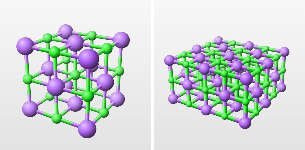
The printed object is the model of the view, without margin, for a chosen number of cells along a, b and c. Laue removes the stubs (the half-bonds to atoms outside the object) and, unless told otherwise, the atoms that no bond holds. Each atom becomes a closed UV sphere (24 meridians, 12 slices). Each bond becomes two closed half-cylinders, each in the colour of its atom, meeting in the middle. All faces are oriented outwards.
The solids overlap, and Laue does not compute their Boolean union: slicers themselves merge the volumes of one part. The scale brings the longest side, radii included, to the requested size. The radius of an atom is as in the view, with a minimum of 1.5 times the radius of a bond. The object is centred and placed on the build plate ().
Laue does not generate supports: slicers compute them better (tree or organic supports, interfaces, soluble material), depending on the printer. The number of parts shown is the number of connected components of the graph of atoms and bonds.
In Laue
STL is binary: 50 bytes per triangle, in millimetres, without colour. 3MF (Core specification of the 3MF Consortium) is an OPC archive containing 3D/3dmodel.model, in unit="millimeter". There is one object per element, linked to a base material that carries the element's colour, and a parent object made of components: slicers open it as a single object with several parts. The tests check that each mesh is closed (each edge traversed once in each direction), that the signed volume is positive, as well as the size, the placement and the absence of stubs.
Saved views and presentation
In Laue
Save View keeps the orientation, the zoom and the display in the document. Present plays them one after the other, for a seminar or a lecture.
References
- International Tables for Crystallography, vol. A, Space-group symmetry, 6th ed., M. I. Aroyo (ed.), IUCr/Wiley, 2016.
- S. R. Hall, “Space-group notation with an explicit origin”, Acta Cryst. A37, 517 (1981).
- C. Giacovazzo (ed.), Fundamentals of Crystallography, 3rd ed., Oxford University Press, 2011.
- D. Waasmaier, A. Kirfel, “New analytical scattering-factor functions for free atoms and ions”, Acta Cryst. A51, 416 (1995).
- B. Cordero et al., “Covalent radii revisited”, Dalton Trans., 2832 (2008).
- W. Friedrich, P. Knipping, M. Laue, “Interferenz-Erscheinungen bei Röntgenstrahlen”, Sitzungsber. Bayer. Akad. Wiss., 303 (1912).
- J. L. Amorós, M. J. Buerger, M. C. Amorós, The Laue Method, Academic Press, 1975.
- W. R. Busing, H. A. Levy, “Angle calculations for 3- and 4-circle X-ray and neutron diffractometers”, Acta Cryst. 22, 457 (1967).
- 3MF Consortium, 3MF Core Specification, version 1.3, 2022.
- V. K. Pecharsky, P. Y. Zavalij, Fundamentals of Powder Diffraction and Structural Characterization of Materials, 2nd ed., Springer, 2009.
- H. M. Rietveld, “A profile refinement method for nuclear and magnetic structures”, J. Appl. Cryst. 2, 65 (1969).
- G. Caglioti, A. Paoletti, F. P. Ricci, Nucl. Instrum. 3, 223 (1958).
- J.-F. Bérar, G. Baldinozzi, “Modeling of line-shape asymmetry in powder diffraction”, J. Appl. Cryst. 26, 128 (1993).
- P. M. de Wolff, “A simplified criterion for the reliability of a powder pattern indexing”, J. Appl. Cryst. 1, 108 (1968).
- M. L. Cohen, T. K. Bergstresser, “Band structures and pseudopotential form factors for fourteen semiconductors of the diamond and zinc-blende structures”, Phys. Rev. 141, 789 (1966).
- W. A. Harrison, Elementary Electronic Structure, World Scientific, 1999.
- J. C. Slater, G. F. Koster, “Simplified LCAO method for the periodic potential problem”, Phys. Rev. 94, 1498 (1954).
- W. Setyawan, S. Curtarolo, “High-throughput electronic band structure calculations: challenges and tools”, Comput. Mater. Sci. 49, 299 (2010).
- P. E. Blöchl, O. Jepsen, O. K. Andersen, “Improved tetrahedron method for Brillouin-zone integrations”, Phys. Rev. B 49, 16223 (1994).
- Z. H. Levine, D. C. Allan, “Linear optical response in silicon and germanium including self-energy effects”, Phys. Rev. Lett. 63, 1719 (1989).
- J. Tauc, R. Grigorovici, A. Vancu, “Optical properties and electronic structure of amorphous germanium”, Phys. Status Solidi 15, 627 (1966).
- P. N. Keating, “Effect of invariance requirements on the elastic strain energy of crystals with application to the diamond structure”, Phys. Rev. 145, 637 (1966).
- R. M. Martin, “Elastic properties of ZnS structure semiconductors”, Phys. Rev. B 1, 4005 (1970).
- G. Nilsson, G. Nelin, “Study of the homology between silicon and germanium by thermal-neutron spectrometry”, Phys. Rev. B 6, 3777 (1972).
- E. W. Kellermann, “Theory of the vibrations of the sodium chloride lattice”, Phil. Trans. R. Soc. Lond. A 238, 513 (1940).
- P. P. Ewald, “Die Berechnung optischer und elektrostatischer Gitterpotentiale”, Ann. Phys. 369, 253 (1921).
- W. L. Bragg, “The refractive indices of calcite and aragonite”, Proc. R. Soc. Lond. A 105, 370 (1924).
- R. H. Lyddane, R. G. Sachs, E. Teller, “On the polar vibrations of alkali halides”, Phys. Rev. 59, 673 (1941).
- J. R. Tessman, A. H. Kahn, W. Shockley, “Electronic polarizabilities of ions in crystals”, Phys. Rev. 92, 890 (1953).
- S. P. S. Porto, R. S. Krishnan, “Raman effect of corundum”, J. Chem. Phys. 47, 1009 (1967).
- Y. Tanabe, S. Sugano, “On the absorption spectra of complex ions”, J. Phys. Soc. Jpn. 9, 753 (1954).
- H. F. Ivey, “Spectral location of the absorption due to color centers in alkali halide crystals”, Phys. Rev. 72, 341 (1947).
- D. S. McClure, “Optical spectra of transition-metal ions in corundum”, J. Chem. Phys. 36, 2757 (1962).
- H. G. Cronemeyer, “Optical absorption characteristics of pink ruby”, J. Opt. Soc. Am. 56, 1703 (1966).
- E. V. Dubinsky, J. Stone-Sundberg, J. L. Emmett, “A quantitative description of the causes of color in corundum”, Gems & Gemology 56, 2 (2020).
- A. B. P. Lever, Inorganic Electronic Spectroscopy, 2nd ed., Elsevier, 1984.
- P. Weiss, “L'hypothèse du champ moléculaire et la propriété ferromagnétique”, J. Phys. Théor. Appl. 6, 661 (1907).
- C. G. Shull, J. S. Smart, “Detection of antiferromagnetism by neutron diffraction”, Phys. Rev. 76, 1256 (1949).
- M. Kohgi, Y. Ishikawa, Y. Endoh, “Inelastic neutron scattering study of spin waves in MnO”, Solid State Commun. 11, 391 (1972).
- M. T. Hutchings, E. J. Samuelsen, “Measurement of spin-wave dispersion in NiO by inelastic neutron scattering and its relation to magnetic properties”, Phys. Rev. B 6, 3447 (1972).
- V. C. Morano, Z. Maesen, S. E. Nikitin, J. Lass, D. G. Mazzone, O. Zaharko, “Absence of altermagnetic magnon band splitting in MnF₂”, arXiv:2412.03545 (2024).
- M. Pajda, J. Kudrnovský, I. Turek, V. Drchal, P. Bruno, “Ab initio calculations of exchange interactions, spin-wave stiffness constants, and Curie temperatures of Fe, Co, and Ni”, Phys. Rev. B 64, 174402 (2001).
- M. Alaei, Z. Mosleh, N. Rezaei, A. R. Oganov, “Experimental exchange interaction dataset for magnetic materials: spin waves to MC simulations”, arXiv:2504.15764 (2025).
- A. B. Pippard, “An experimental determination of the Fermi surface in copper”, Phil. Trans. R. Soc. Lond. A 250, 325 (1957).
- W. A. Harrison, “Electronic structure of polyvalent metals”, Phys. Rev. 118, 1190 (1960).
- N. W. Ashcroft, N. D. Mermin, Solid State Physics, Holt, Rinehart and Winston, 1976.
- D. B. Litvin, Magnetic Group Tables, IUCr, 2013.
- H. T. Stokes, D. M. Hatch, B. J. Campbell, ISO-MAG, ISOTROPY Software Suite, iso.byu.edu (version 1.4, 2022).
- O. Halpern, M. H. Johnson, “On the magnetic scattering of neutrons”, Phys. Rev. 55, 898 (1939).
- P. J. Brown, “Magnetic form factors”, International Tables for Crystallography, vol. C, § 4.4.5.
- T. Holstein, H. Primakoff, “Field dependence of the intrinsic domain magnetization of a ferromagnet”, Phys. Rev. 58, 1098 (1940).
- L. Nordheim, “Zur Elektronentheorie der Metalle. I”, Ann. Phys. 401, 607 (1931).
- R. Braunstein, A. R. Moore, F. Herman, “Intrinsic optical absorption in germanium-silicon alloys”, Phys. Rev. 109, 695 (1958).
- A. Zunger, S.-H. Wei, L. G. Ferreira, J. E. Bernard, “Special quasirandom structures”, Phys. Rev. Lett. 65, 353 (1990).
- J. H. P. Colpa, “Diagonalization of the quadratic boson Hamiltonian”, Physica A 93, 327 (1978).
- G. P. Felcher, R. Kleb, “Antiferromagnetic domains and the spin-flop transition of MnF2”, Europhys. Lett. 36, 455 (1996).
- I. E. Dzyaloshinskii, “On the magneto-electrical effect in antiferromagnets”, Sov. Phys. JETP 10, 628 (1960).
- D. N. Astrov, “The magnetoelectric effect in antiferromagnetics”, Sov. Phys. JETP 11, 708 (1960).
- P. J. Brown, J. B. Forsyth, F. Tasset, “A study of magnetoelectric domain formation in Cr2O3”, J. Phys.: Condens. Matter 14, 1957 (2002).
- S. Sugano, Y. Tanabe, “Absorption spectra of Cr3+ in Al2O3. Part A”, J. Phys. Soc. Jpn. 13, 880 (1958).
- V. K. Sewani et al., “Spin thermometry and spin relaxation of optically detected Cr3+ ions in ruby Al2O3”, Phys. Rev. B 102, 104114 (2020).
- M. Gen et al., “Crystal-field Paschen-Back effect on ruby in ultrahigh magnetic fields”, Phys. Rev. Research 2, 033257 (2020).
- R. G. Burns, Mineralogical Applications of Crystal Field Theory, 2nd ed., Cambridge University Press, 1993.
- K. Nassau, The Physics and Chemistry of Color, 2nd ed., Wiley, 2001.
- C. Wyman, P.-P. Sloan, P. Shirley, “Simple analytic approximations to the CIE XYZ color matching functions”, J. Comput. Graph. Tech. 2, 1 (2013).
- O. Madelung, Semiconductors: Data Handbook, 3rd ed., Springer, 2004.
- P. Y. Yu, M. Cardona, Fundamentals of Semiconductors, 4th ed., Springer, 2010.
- J. H. Conway, H. Burgiel, C. Goodman-Strauss, The Symmetries of Things, A K Peters, 2008.
- M. Baake, U. Grimm, Aperiodic Order, vol. 1, Cambridge University Press, 2013.
- N. G. de Bruijn, “Algebraic theory of Penrose's non-periodic tilings of the plane”, Indag. Math. 43, 39 (1981).
- M. Baake, R. V. Moody, P. A. B. Pleasants, “Diffraction from visible lattice points and k-th power free integers”, Discrete Math. 221, 3 (2000).
- D. Shechtman, I. Blech, D. Gratias, J. W. Cahn, Phys. Rev. Lett. 53, 1951 (1984).
- P. J. Lu, P. J. Steinhardt, “Decagonal and quasi-crystalline tilings in medieval Islamic architecture”, Science 315, 1106 (2007).