 Laue
Guide — Teaching
This guide is a manual. Each chapter begins with the theory: what we are trying to describe, why we describe it that way, and what you need to know to understand what the app shows. It goes on with the practice: where to find it in Laue and how to use it. You can read the chapters in order, as a short course, or go straight to the one you need. The “In class” boxes suggest an activity and point out the difficulties pupils and students usually meet.
Before you start: documents, examples and settings
In Laue
Laue works on documents of three kinds, each opened in its own workshop: a crystal (in three dimensions), a plane pattern (tiling, frieze or mandala) and a quasicrystal. The toolbar menu New creates one or the other. If the window is still empty, the new document takes its place; otherwise it opens in a new window. This behaviour can be changed in the settings.
A document is saved in the .laue format, a readable text file, the same on Mac, on iPad and on PC, whose description is published. Every change can be undone and redone with the toolbar buttons, whose tooltip says what they are about to undo.
The Examples button opens the library, which has two shelves: Examples (thirteen crystals, tilings, mandalas, quasicrystals) and Exercises (Tutor). The list on the left shows the titles at a glance; a click shows the description on the right, and Open opens it as a copy, in the language of the interface. Nothing can be damaged.
The settings (Laue › Settings menu on Mac, the gear wheel on iPad) begin with the Usage, asked at first launch. Design names the symmetries in words and shows the pattern alone, Teaching shows symbols and symmetry elements, and Science gives the international symbols and the diffraction. No feature is removed: only what is shown first changes. The settings also set what a new document creates, how the 3D view looks when it opens, how coordinates are written (decimals or fractions), the resolution of exported images, the starting values of the powder pattern, and the folders for opening and saving.
The Crystal workshop: the sidebar
In Laue
To the left of a crystal's 3D view, the sidebar arranges its settings in five tabs, chosen with the icons at the top; the name of the open tab is shown below them, and each window keeps its own.
- Construction: what the crystal is — the space group, the cell, the sites and their Wyckoff positions, the composition, the online reference values and the checks of an exercise. Choosing an atom, in the list or in the view, brings you back to this tab, on its inspector.
- Diffraction: the stereogram of the crystal class, the powder pattern and the Laue pattern.
- Properties: the band structure, with its phonons and its optics, and the colour centres.
- Simulations: magnetism, from the mean field to thermal agitation.
- View: what is shown and how — the cells, filling the view, the size of the atoms, the bonds, the polyhedra, the perspective, the zoom, the symmetry elements, looking along an axis, the orientation to the degree (the polar angle θ and the azimuth φ of the direction towards you in the crystal's frame, and a turn ψ about it, set with the slider or typed in) and the presentation views.
An exercise that asks you to find the diffraction hides it: the Diffraction tab then keeps only the stereogram.
The lattice and the cell
What the theory says
A crystal is an arrangement of atoms that repeats identically in all three directions of space. To describe it without listing billions of atoms, we split it into two ideas.
- The lattice is the set of translations that leave the crystal unchanged. These are points, without atoms: all the places where exactly the same surroundings are found.
- The motif is what is placed at each lattice point: an atom, a molecule, a group of atoms.
Three vectors a, b, c generate the lattice, and the parallelepiped they span is the cell. Its six parameters (the lengths a, b, c and the angles α, β, γ) and the coordinates of the atoms in the cell, as fractions of these vectors, are enough to rebuild the whole crystal. This is the great economy of crystallography.
There are infinitely many ways of choosing three vectors that generate the same lattice. One is chosen according to two criteria that sometimes pull in opposite directions:
- the primitive cell contains only one lattice point: it is as small as possible;
- the conventional cell follows the symmetry, at the cost of sometimes being larger. The cell of rock salt is a cube containing four lattice points (a “face-centred cubic” lattice); its primitive cell would be a rhombohedron with 60° angles, which hides the cubic symmetry.
The International Tables, and therefore Laue, use the conventional cell. The fourteen ways of arranging lattice points in space are the Bravais lattices: primitive (P), body-centred (I), face-centred (F), one-face-centred (A, B or C) and rhombohedral (R), across the seven crystal systems. The system constrains the cell: a = b = c and all angles right angles for a cube, a = b and γ = 120° for a hexagonal lattice, and so on.
The formulas
A lattice point, and an arbitrary point in fractional coordinates:
The metric tensor contains the six cell parameters; it gives distances, angles and the volume:
In Laue
In the Crystal workshop, on the Construction tab, the Cell section shows only the parameters the crystal system leaves free: a alone for a cubic group, a and c for a tetragonal or hexagonal group, all six for a triclinic group. Changing the group adapts the cell. Below the fields, Laue recalls the full six parameters. On the View tab, Cells shows 1, 2 or 3 cells in each direction, and Fill the view shows a macroscopic crystal around one cell, drawn in the centre: the lattice reaches the edges of the view, and the number of cells no longer counts; when zooming out on a large structure, Fade with the distance blends the distant atoms into the background.
Symmetry and point groups
What the theory says
A symmetry operation is a motion that leaves the object unchanged: a rotation, a mirror, an inversion through a point, or a combination. The set of operations of an object forms a group: performing two symmetries in succession again gives a symmetry, and each one can be undone.
Periodicity imposes a strong constraint, the crystallographic restriction: a lattice can only have rotation axes of order 1, 2, 3, 4 or 6. The reason is simple. Expressed in the lattice basis, a rotation that maps the lattice onto itself has integer coefficients; so its trace is an integer too. But the trace of a rotation through 2π/n is 1 + 2 cos(2π/n), which is an integer only for n = 1, 2, 3, 4 or 6. No crystal of order 5, and no tiling of regular pentagons.
The rotations, mirrors and inversions that leave a point fixed form the point group. It describes the crystal seen from afar, without seeing its atoms: the shape of its faces, and the anisotropy of its properties. Because of the restriction there are only 32 of them, divided among 7 crystal systems, from triclinic to cubic. According to Neumann's principle, every physical property of a crystal has at least the symmetry of its point group. A cubic crystal is therefore optically isotropic, and piezoelectricity requires the absence of a centre of symmetry.
A point group is drawn in stereographic projection. The crystal is surrounded by a sphere, the points where its axes and mirrors pierce the sphere are marked, and the result is projected onto the equatorial plane. An arbitrary direction appears there with all its copies: 48 for the cubic group m-3m, as many equivalent orientations.
The formulas
The crystallographic restriction: in a lattice basis, the rotation is a matrix of integers, so its trace is an integer too.
In Laue
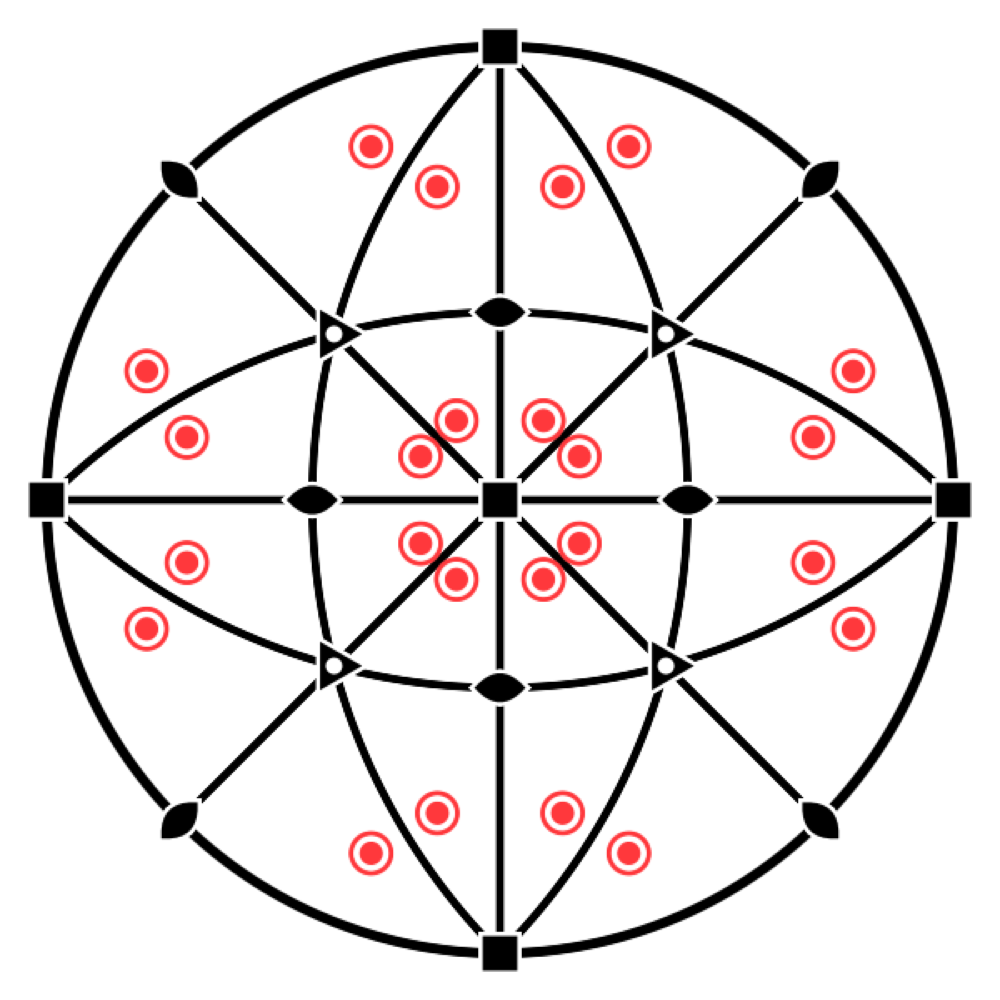
In the Crystal workshop, the Stereogram switch places that of the point group below the view, with its elements and the equivalent positions. When a site is selected, the stereogram shows its own symmetry, the site symmetry. It is the quickest way to see why an atom of diamond has site symmetry -43m and not m-3m: it lacks the centre of inversion.
Space groups
What the theory says
The space group brings together the lattice and the point group, and describes the full symmetry of the atomic arrangement. It adds operations with no point-group counterpart, because they combine a rotation or a mirror with a fraction of a translation:
- a screw axis nₖ turns through 360°/n and then advances by k/n of the period, like a spiral staircase (2₁, 3₁, 4₂, 6₅…);
- a glide plane reflects and then shifts by half a translation, like footprints in the snow (a, b, c, n, d, e).
Each operation is written {R | t}: a linear part R followed by a translation t (Seitz notation). There are 230 space groups. The Hermann–Mauguin symbol names them as follows: first the lattice letter (P, I, F…), then the symmetry elements along the principal directions. Thus Fm-3m is the group of rock salt, and P2₁/c that of many molecular crystals. Depending on the choice of axes and origin, the same group can be written in several ways: the Tables list 530 “settings”, and the Hall symbol describes each of them unambiguously.
The formulas
An operation in Seitz notation:
A 4₂ axis along c, for example: a quarter turn, then half a step along the axis.
In Laue
The group field takes a number (227), a short or full Hermann–Mauguin symbol (Fd-3m, P2_1/c), a setting (227:1) or a Hall symbol (Hall: -P 2ybc). All 530 settings of the Tables are recognised, and the list next to the field offers them all.
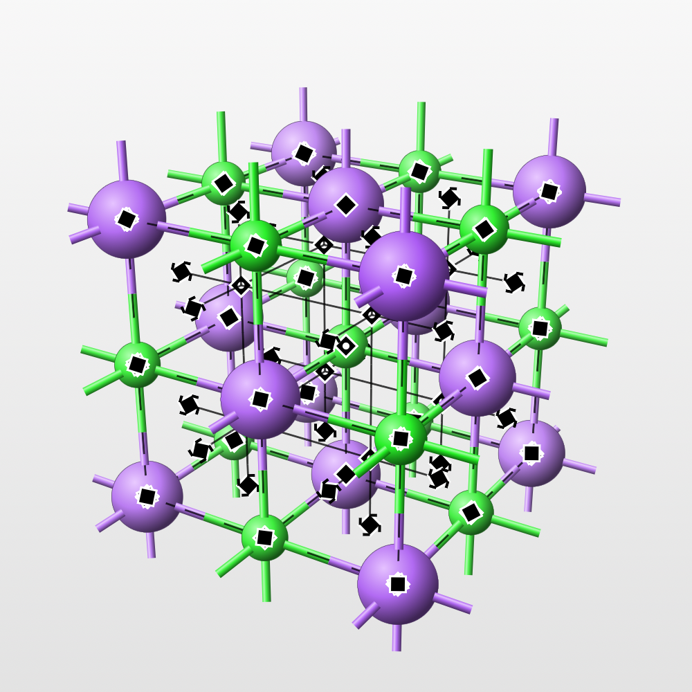
Symmetry elements are drawn in the 3D view with the symbols of the Tables: rotation and screw axes, rotoinversion axes, mirror and glide planes, inversion centres. You choose which to show in Symmetry elements. Since a cubic cell has dozens of axes, the Orders row lets you show just one order at a time (2, 3, 4 or 6). The elements pass behind the atoms like everything else.
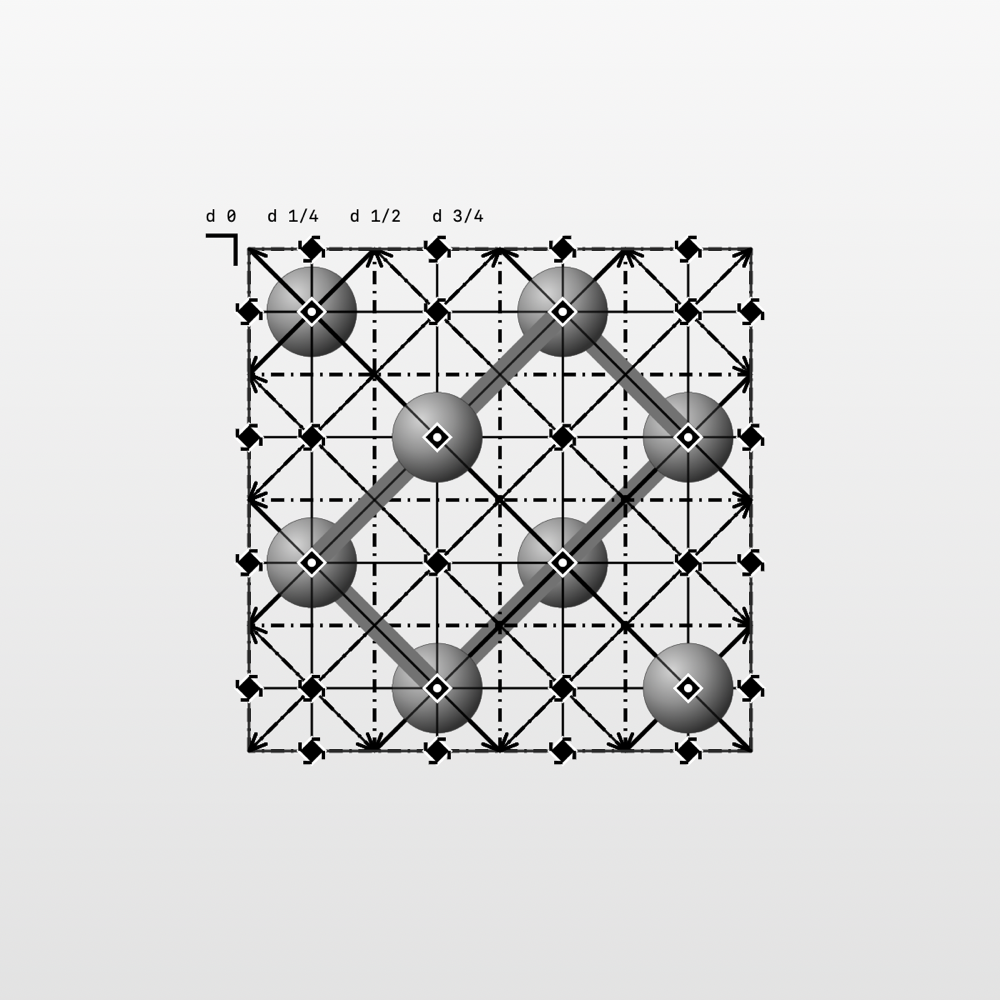
Look along turns the view onto a lattice direction or onto a symmetry element. The Projection of the Tables reproduces the diagrams of Volume A of the International Tables, with the heights of the planes. Drag to turn, pinch to zoom, and choose between orthographic view and perspective.
The symbols of the Tables
What the Tables say
The diagrams of Volume A of the International Tables represent each symmetry element by a graphical symbol (section 1.4 of the 2006 edition, chapter 2.1 of the 2016 edition: they are the same). Laue draws these symbols in the 3D view, the projection of the Tables, the stereograms and the tilings; the figures in these tables come from the same library as the app. The notation is that of the Tables, with partial elements in parentheses; the intrinsic translation is given as a fraction of the shortest lattice translation along the axis or the glide.
Axes perpendicular to the drawing, symmetry points
| Symbol | Element | Notation | Intrinsic translation |
|---|---|---|---|
 | Twofold rotation axis; twofold point in the plane | 2 | — |
 | Screw axis 2₁ | 2₁ | |
 | Threefold rotation axis; threefold point in the plane | 3 | — |
 | Screw axis 3₁ | 3₁ | |
 | Screw axis 3₂ | 3₂ | |
 | Fourfold rotation axis; fourfold point in the plane | 4 (2) | — |
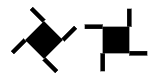 | Screw axis 4₁ | 4₁ (2₁) | |
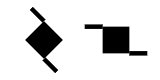 | Screw axis 4₂ | 4₂ (2) | |
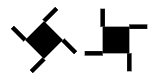 | Screw axis 4₃ | 4₃ (2₁) | |
 | Sixfold rotation axis; sixfold point in the plane | 6 (3, 2) | — |
 | Screw axis 6₁ | 6₁ (3₁, 2₁) | |
 | Screw axis 6₂ | 6₂ (3₂, 2) | |
 | Screw axis 6₃ | 6₃ (3, 2₁) | |
 | Screw axis 6₄ | 6₄ (3₁, 2) | |
 | Screw axis 6₅ | 6₅ (3₂, 2₁) | |
 | Inversion centre | — | |
 | Rotoinversion axis 3̄ | (3, ) | — |
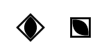 | Rotoinversion axis 4̄ | (2) | — |
 | Rotoinversion axis 6̄ | — | |
 | Twofold axis with an inversion centre | 2/m () | — |
 | Screw axis 2₁ with an inversion centre | 2₁/m () | |
 | Fourfold axis with an inversion centre | 4/m (, 2, ) | — |
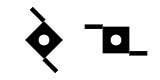 | Screw axis 4₂ with an inversion centre | 4₂/m (, 2, ) | |
 | Sixfold axis with an inversion centre | 6/m (, , 3, 2, ) | — |
 | Screw axis 6₃ with an inversion centre | 6₃/m (, , 3, 2₁, ) |
The tails of a screw axis extend its sides. An axis nₖ carries n/gcd(n, k) of them: 4₂ has two, 6₂ and 6₄ three, 6₃ two, matching the partial elements 2, 3₂, 3₁ and 2₁ they contain. Their sense is reversed between enantiomorphic axes: 3₁ and 3₂, 4₁ and 4₃, 6₁ and 6₅, 6₂ and 6₄. The symbol of a fourfold axis is drawn as a diamond or with its sides parallel to the cell edges. An inversion centre lying on the axis gives the symbol n/m, marked with a white dot; on a 4₂ or 6₃ axis, the 4̄ and 6̄ points are not marked.
Twofold axes lying in the drawing
| Symbol | Element | Notation | Intrinsic translation |
|---|---|---|---|
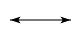 | Twofold rotation axis | 2 | — |
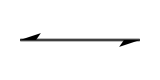 | Screw axis 2₁ | 2₁ |
Planes perpendicular to the drawing, symmetry lines
| Symbol | Element | Notation | Intrinsic translation |
|---|---|---|---|
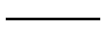 | Mirror plane; reflection line in the plane | m | — |
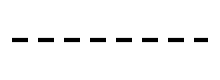 | “Axial” glide plane, glide in the drawing; glide line in the plane | a, b or c; g | of a translation along the line |
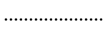 | “Axial” glide plane, glide towards the viewer | a, b or c | of a translation perpendicular to the drawing |
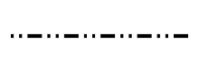 | “Double” glide plane (centred cells) | e | two glides: along the line and perpendicular to the drawing |
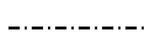 | “Diagonal” glide plane | n | one glide with two components, along the line and perpendicular to it |
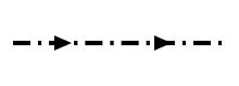 | “Diamond” glide plane (pair of planes, centred cells) | d | along the line and perpendicular to it; the arrow shows the direction in the drawing for which the perpendicular component is positive |
For a, b, c and n, the line style depends on the direction of the glide relative to the drawing, not on the letter: the same dotted line is a c plane in one description and an n plane in another (R3̄c in hexagonal or rhombohedral axes).
Planes parallel to the drawing
| Symbol | Element | Notation | Intrinsic translation |
|---|---|---|---|
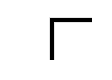 | Mirror plane | m | — |
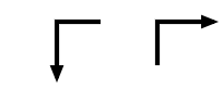 | “Axial” glide plane | a, b or c | of a translation in the direction of the arrow |
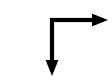 | “Double” glide plane (centred cells) | e | in the direction of either arrow |
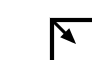 | “Diagonal” glide plane | n | in the direction of the arrow |
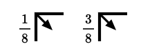 | “Diamond” glide plane (pair of planes, centred cells) | d | in the direction of the arrow, that is a quarter of a diagonal of the face-centred cell |
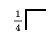 | A mirror plane at heights and | m | — |
These symbols are placed at the top left of the diagram, their branches along the cell edges. A fraction h denotes the pair of planes at heights h and h + ½; without a fraction, the planes are at heights 0 and ½.
In Laue
The Projection of the Tables looks at the cell from the side the chosen direction points to, like the diagrams: along c, a points down and b to the right, and a screw axis turns in the same sense as in the Tables. Leave the pointer on an element for a moment: a tooltip names it and gives its direction, its position () and its intrinsic translation; if several elements overlap, it lists them all.
Wyckoff positions
What the theory says
An atom placed anywhere in the cell is copied by all the operations of the group: this is its orbit. But if it is placed on a symmetry element (a mirror, an axis, a centre), some operations leave it where it is. Its copies then coincide in twos or threes, and it has fewer of them. The operations that leave it in place form its site symmetry.
The Wyckoff positions classify the points of the cell by this local symmetry. Each has a letter (a, b, c…, from the most symmetric to the least), a multiplicity (the number of copies in the conventional cell) and a site symmetry. The multiplicity times the order of the site symmetry is the same for all the positions of a group. The fewer copies, the more symmetric the site.
This is the language of structure descriptions: “Na on 4a, Cl on 4b” is enough to describe rock salt, because the group Fm-3m does the rest. A general position has three free coordinates; a special position has fewer, or none, and its coordinates are then fixed by symmetry.
The formulas
For a position of multiplicity and site symmetry , in a group with point group and a cell with lattice points (1 for P, 2 for I and C, 4 for F):
For rock salt, in : Na on 4a, ; a general position 192l, .
In Laue
Add a site creates an atom, named after its element (Ca1, O1), a name you can change; you choose its element and its coordinates, with the slider or by typing their value in the field at the end of each slider. Coordinates are written exactly, for example 1/3 or 0.4697, and Laue keeps them exact. The site inspector gives its Wyckoff position (8a, 24d…), its multiplicity and its oriented site symmetry. Put on a Wyckoff position offers the positions of the group. With the move tool, you drag an atom in the 3D view: it snaps onto the special positions it crosses, and Stay on keeps it on its position while it slides along it. All its copies follow. Two atoms closer than any bond are flagged: most often a coordinate left at its starting value, or a cell edge that was not set (the c of a hexagonal group left equal to a).
Atoms and composition
What the theory says
The motif is made of atoms, and each chemical element has its own characteristics. Its atomic number Z (the number of protons) identifies it; its atomic mass weighs the cell. Its electron configuration and its electronegativity say how it bonds. Its covalent radius gives the typical length of its bonds, and its oxidation states the charges it takes in an ionic compound.
Counting the atoms in the cell gives the formula of the crystal and the number Z of formula units per cell: four NaCl in the cell of rock salt. The mass of the cell divided by its volume gives the density, a simple and valuable check on a structure: a calculated density far from the measured one signals an error.
The formulas
The density, with units of molar mass in a cell of volume (: Avogadro's number):
For rock salt ( = 5.640 Å):
In Laue
In a site's inspector, the grid button next to the Element field opens the periodic table: the 103 elements in their usual colours. Hovering shows an element's card (atomic number and mass, electron configuration, electronegativity, covalent radius, oxidation states), and a click selects it. You can also type the symbol; an unknown symbol is flagged.
The Composition section of the Construction tab gives the formula, Z, the molar mass and the density. In the 3D view, the size of the atoms and the bonds follow the covalent radii. Bonds that leave the cells are hidden; untick Hide the bonds leaving the cells to see them and read the full coordination of each atom. Two ions of the same sign are never bonded.
A site can be shared: in an alloy or a solid solution, several elements occupy the same positions at random, each with its own fraction — in the example Al₀.₃Ga₀.₇As, 70 % gallium and 30 % aluminium on the cation site. In the site's inspector, Share this site with another element adds an element and its fraction; with two elements, changing one changes the other, and fractions whose sum stays below 1 leave part of the sites empty (vacancies). The formula, the density and the diffraction patterns take this into account, CIF import and export read and write the occupancies, and the 3D view draws these atoms with an averaged colour and size.
Coordination polyhedra, in the display settings, surrounds each central atom with the polyhedron of its neighbours, with translucent faces in its colour: the SiO₄ tetrahedra of quartz, the TiO₆ octahedra of perovskite and rutile, the CaF₈ cubes of fluorite. The polyhedron follows its neighbours outside the cell, and the bonds it contains disappear. By default, the centres are the atoms surrounded by four to eight neighbours more electronegative than themselves; the Centres menu chooses others.
The Measure tool (the ruler, beside Turn and Move atoms) measures between the atoms of the 3D view. Click two atoms for their distance, three for the angle at the second, four for the torsion, signed as IUPAC has it. From three atoms on, the Measurements panel also gives their mean plane, with its indices (hkl) when the atoms truly lie in it, and each one's deviation. A single atom gives its nearest neighbours and their distances. The atoms picked are numbered and joined in the view; clicking an atom again drops it, clicking the background clears them all, and Copy gives the measurements as text, for a spreadsheet.
The Bond valence sums section of the Construction tab checks an ionic structure at a glance. Each bond between a cation and an anion carries a valence, exp((R₀ − R)/b), and an ion's bonds add up to its oxidation state: 2.97 for the aluminium of corundum, 0.98 for the sodium of rock salt. R₀ and b are those published for the pair, and the section cites the papers: for oxides, Gagné and Hawthorne (2015) where their comparison over thousands of structures finds them better, otherwise Brown and Altermatt (1985) or another paper; failing that, an estimate from the two elements (O'Keeffe and Brese 1991). A sum more than 0.25 away from the oxidation state is in orange: a bond too long or too short, an atom misplaced, a wrong element. The Global instability index sums up the cell: under 0.1 the structure is unstrained; above 0.2 it is seldom stable.
Structure files
What the theory says
Published structures are exchanged in a handful of formats. CIF (Crystallographic Information File) is the standard of the International Union of Crystallography and of the databases. SHELX (.res, .ins) is the format of single-crystal refinement programs, and POSCAR that of the VASP computational code, which gives every atom but not the group. A file rounds the coordinates (0.666667 instead of 2/3) and does not always state the group in the same way: reading it back correctly means recovering the symmetry.
In Laue
The Structure menu reads a CIF, a SHELX file or a POSCAR. For a CIF, the group is recognised from its symmetry operations, otherwise from its Hall symbol, otherwise from its Hermann–Mauguin symbol. The rounded coordinates recover their exact value, and the atoms settle on their special positions. A POSCAR gets its symmetry back. The same menu writes the structure as CIF, SHELX, POSCAR, extended XYZ or PDB, and its net as CGD, which Systre and the RCSR database read to name a topology (dia, pcu…).
In the Construction tab, the Supercell and slab section remakes the crystal in P1, every atom a site of its own: to put a defect, a substitution or some disorder in it, or to export it to a calculation code. A supercell repeats the cell n₁ × n₂ × n₃ times. A slab cuts the crystal parallel to the plane (hkl): you choose the number of layers, one period of the plane each, and the vacuum above; a and b lie in the plane and c is perpendicular to it, as surface calculations expect. Undo brings the original crystal back.
Tilings: the 17 plane groups
What the theory says
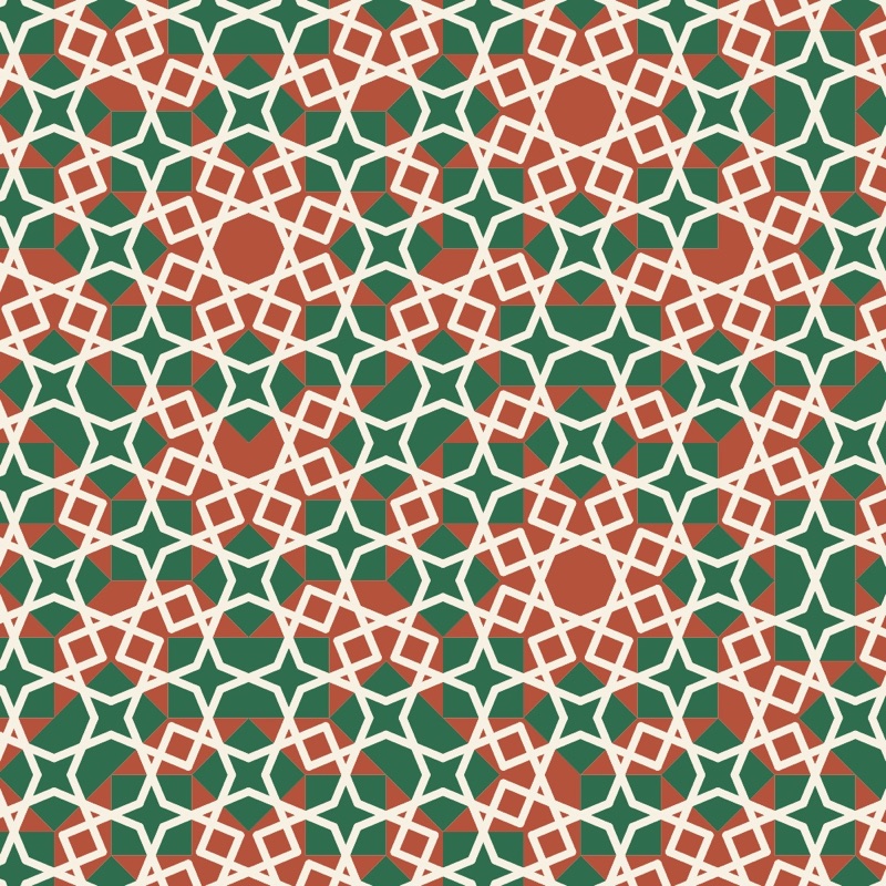
A wallpaper, a tiled floor, a printed fabric: they all repeat a motif in two directions of the plane. They are two-dimensional crystals, and the same theory applies to them, in a simpler form. The motif can be turned, reflected in a mirror, shifted, or these moves can be combined, and the crystallographic restriction allows only rotations of order 2, 3, 4 and 6. The result is exactly seventeen plane groups, proved in the nineteenth century and all present, it is said, in the decoration of the Alhambra.
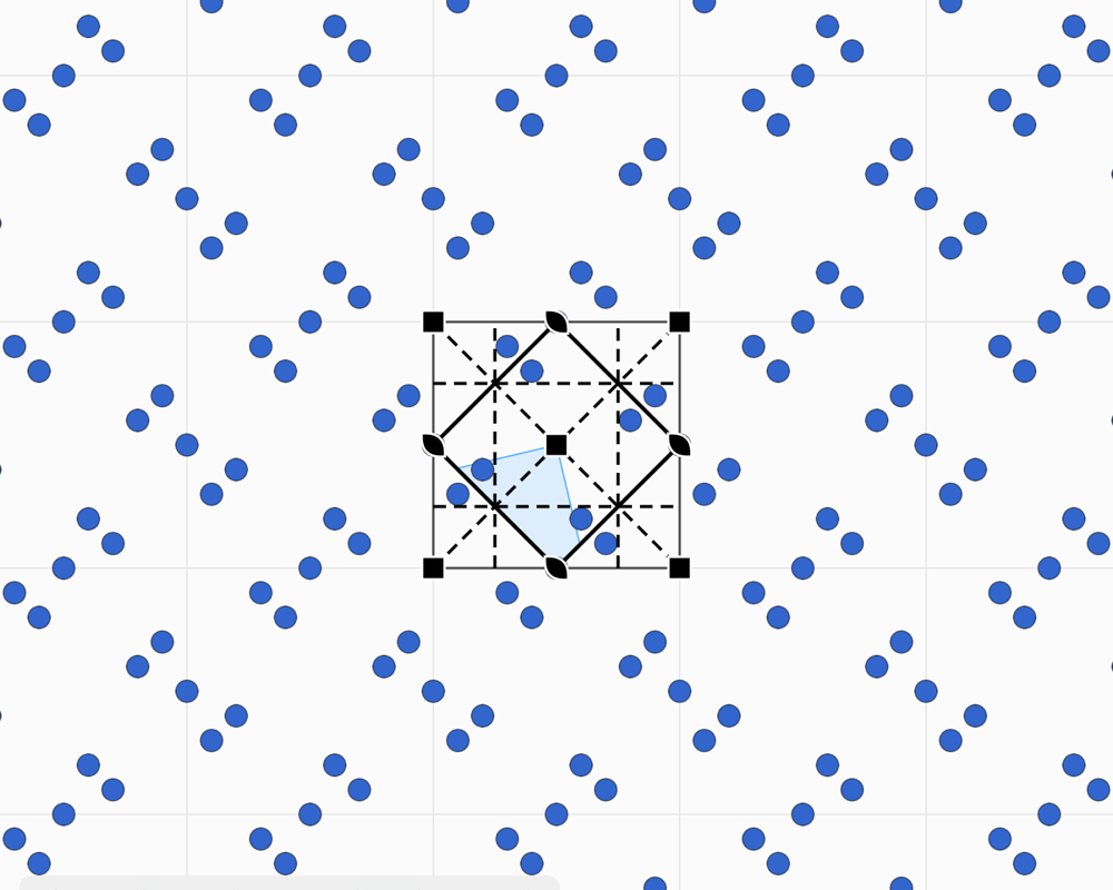
Each group has its fundamental domain: the smallest part of the plane from which the operations rebuild the whole pattern. Drawing in this domain means drawing the whole tiling. The groups are named in two ways. The international symbol, such as p4mm, gives the lattice and then the elements along the directions. Conway's orbifold notation, such as *442, counts the centres of rotation and the mirrors from the topology of the domain.
Two ideas enrich the picture. The two-colour groups (46 in the plane) make a copy change colour under certain operations, as in Escher's prints where a white fish becomes black. Subgroups remove operations: going from p4mm to p4, the mirror copies vanish, and the motif is no longer reflected.
In Laue: step by step
- Choose a rule. At the top of the panel, the Tiling | Frieze | Rosette selector chooses between the 17 plane groups, the 7 friezes, patterns that repeat in one direction only, like a border, and the rosettes, which turn around a point; the Group menu below offers the groups of the chosen kind. To start with, p4mm gives a square kaleidoscope, p6m a hexagonal kaleidoscope, and p4 or p6 a rosette that turns without mirrors.
- Draw in the shaded area. This is the “fundamental domain”, the smallest part of the pattern: everything you draw there is copied everywhere. The Draw tool draws freehand, in the colour you chose.
- Place motifs. The Motif tool places a shape (circle, triangle, square, rhombus, pentagon, hexagon, star, arrow), a letter, a symbol, an emoji or your own picture. The Appearance panel sets its size and rotation. Near a centre of rotation or a mirror, the motif snaps to it, and its copies meet in a rosette.
- Pick the colours. Every stroke and every motif has its own colour, and the background colour can be set too. Two colours picks one of the 46 two-colour groups: the copies change colour under the operations drawn in red.
- Look at the result on its own. Pattern only hides the cell, the lattice and the symbols: only the pattern remains.
- Print or export. As an image for the screen, as a PDF for paper, or for fabric and wallpaper with a seamless repeat (see Printing and fabric).
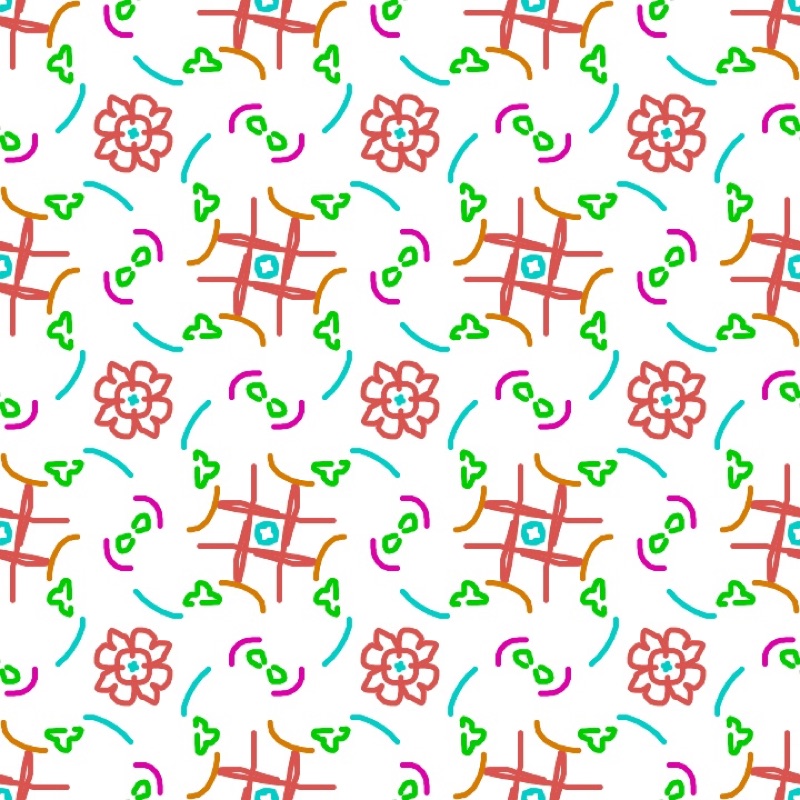
Changing the rule does not change your drawing: it is simply repeated differently. The same freehand stroke becomes a rosette, a kaleidoscope or a scattered pattern depending on the group you choose.
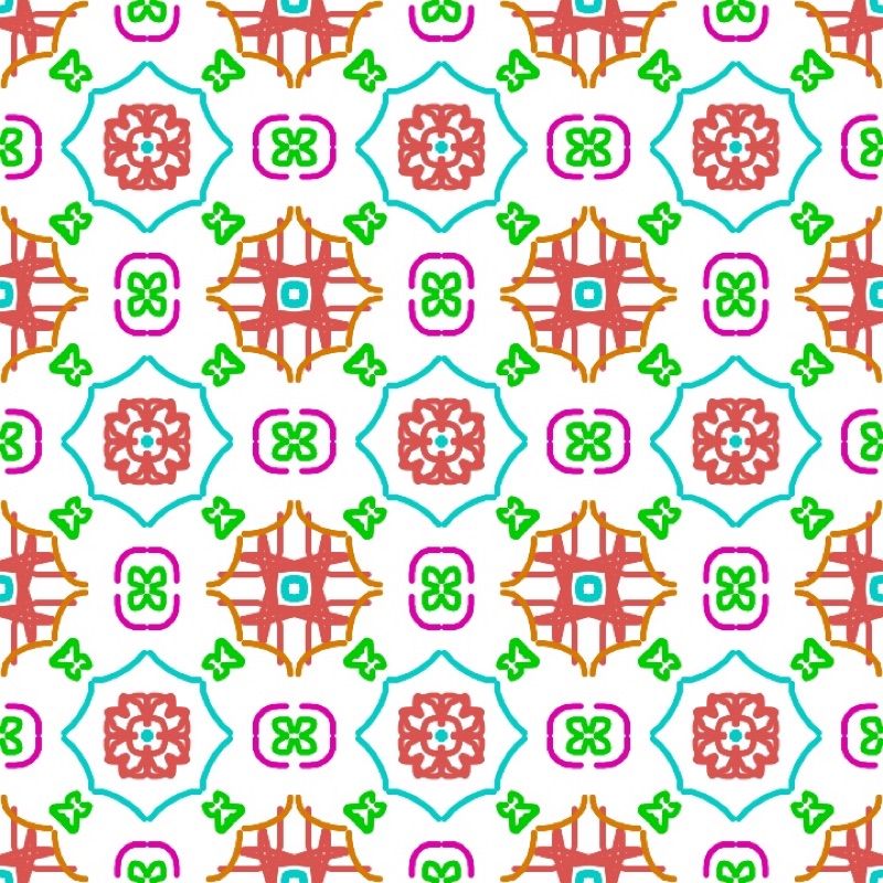
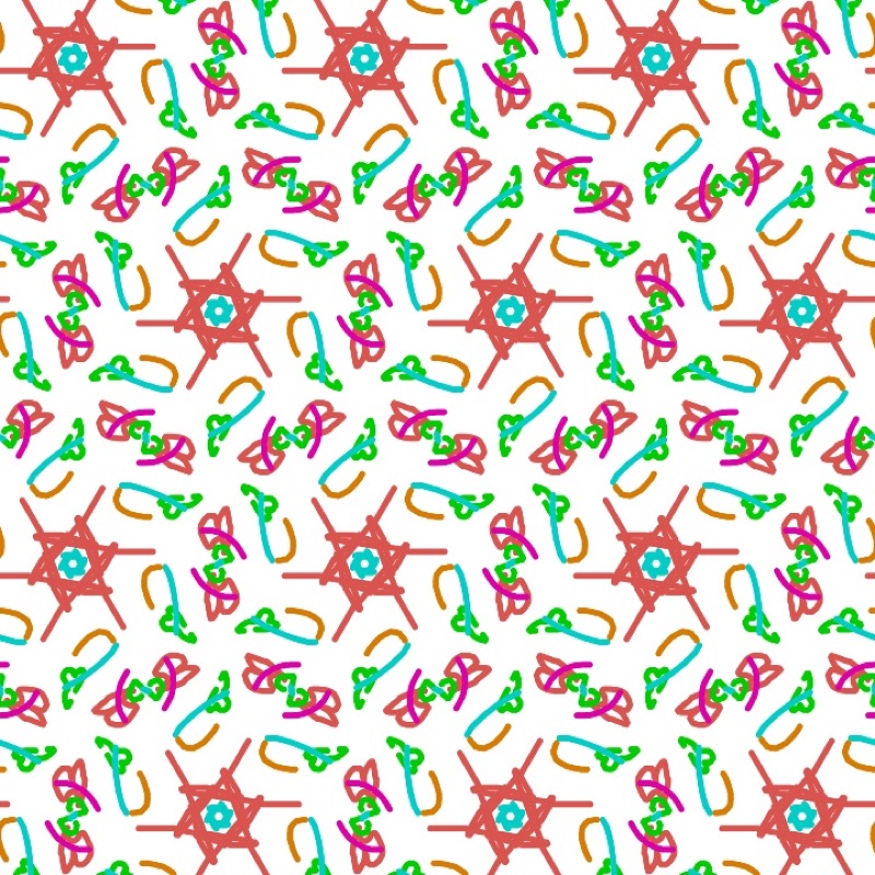
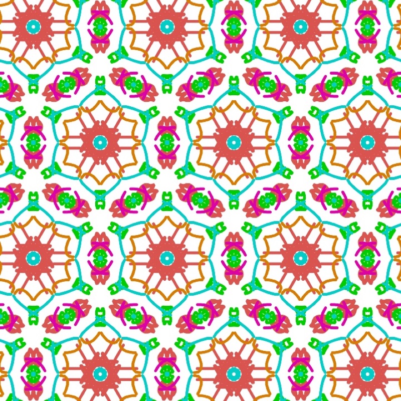
There are four tools. Select moves a motif or a stroke with all its copies, Motif places a motif, Draw draws freehand and Erase erases whatever it touches. An asymmetric motif, such as the letter F, shows what each operation does: turned by the rotations, flipped by the mirrors. On a special position the copies overlap, and a motif with less symmetry than its site makes this visible. The side panel lists the operations of the group and offers its subgroups and supergroups with the same cell. In Display, the Extent shows the Whole plane (the default) or a Portion of columns × rows of cells, from 1 × 1 to 12 × 12, framed and cut at the cell edges: useful for showing a single cell, or a 2 × 2 block on the board.
Finding the rule of a tiled floor. Place a photograph of a floor, a fabric or a print under the pattern. Adjust its position, size, rotation and opacity, and line the cell up with the repeat in the photo. Then try the groups until the symbols land on the centres and mirrors of the original. The tutor's identification exercises train the eye.
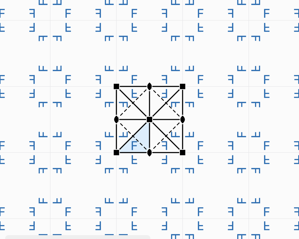
Friezes: the 7 groups of a strip
What the theory says
A frieze, a border, a piece of embroidery or a row of tiles repeats in one direction only. The possible symmetries of a strip are fewer: just seven groups. Conway gave them names you can remember while walking, after the tracks they would leave: the hop, the step, the sidle, the spinning hop… The frieze p11g, for example, is the trail of footprints in the snow, a glide along the strip.
In Laue
The Tiling | Frieze | Rosette selector switches to friezes; the Group menu then offers all seven, with their symbol, their orbifold and their Conway name. The strip is drawn with a height equal to the cell parameter b. All the tiling tools apply to it.
Mandalas and rosettes
What the theory says
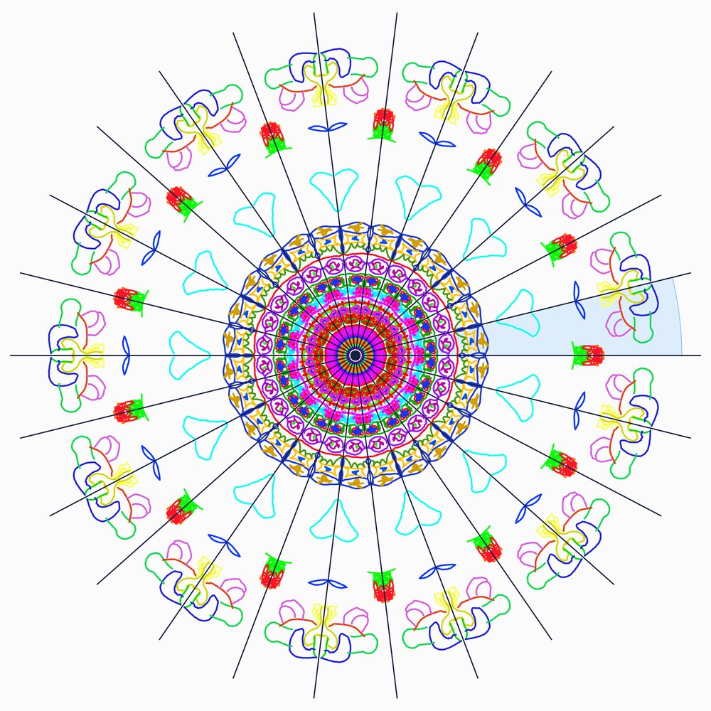
A rosette, a stained-glass window, a flower, a mandala do not repeat across the whole plane: their motif turns around a point. Leonardo da Vinci had noticed that a finite figure has only two kinds of symmetry:
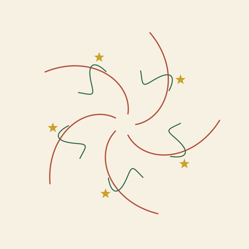
- Cₙ: n rotations only. The arms all turn the same way, like a pinwheel.
- Dₙ: n rotations and n mirrors through the centre, like a star or a cathedral rose window.
Unlike tilings, any order is allowed: 5, 8, 12 or 13. This is the crystallographic restriction seen from the other side. A single figure can have five-fold symmetry; a periodic tiling never can. Penrose's quasicrystals, for their part, have rosettes of order 5 or 10 at their centre.
In Laue
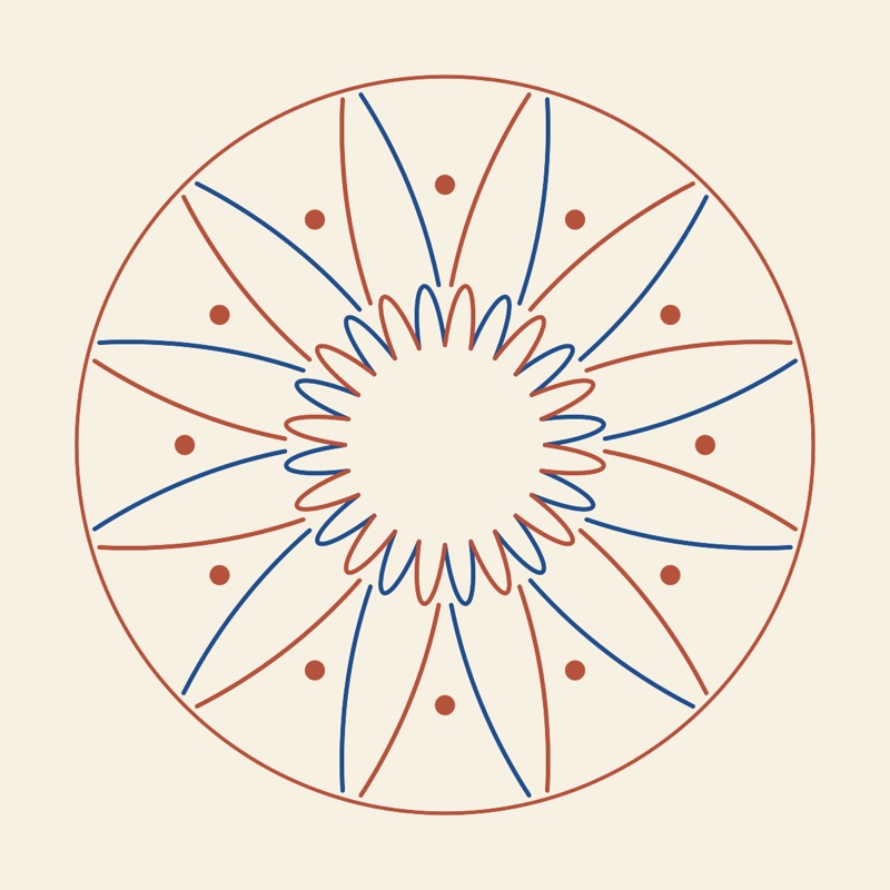
The Tiling | Frieze | Rosette selector (“Mandala” when the usage is Design) opens the workshop. The Order stepper sets n, from 1 to 24, and the Mirrors switch goes from Cₙ to Dₙ. Draw or place a motif in the shaded sector, the fundamental domain: every stroke is copied around the centre. A motif placed on a mirror or at the centre snaps to it and has fewer copies, as the list of motifs shows (site symmetry and number of copies). Zoom, or pinching, enlarges the figure to draw the details. The mirrors guide your hand; Symmetry elements hides them. Two colours alternates the sectors, and the picture exports as PNG or as vector PDF. The thickness and style of the strokes (solid, dashed, dotted, sand powder with its fall radius) are set under the list of lines, in the Tiling and Rosette workshops.
Diffraction
What the theory says
The distances between atoms, of the order of an ångström (10−10 m), are a thousand times too small for visible light. The crystal is therefore illuminated with a wave of comparable wavelength: X-rays, neutrons or electrons. Each atom scatters a little of the wave. Because the crystal is periodic, these waves add up only in certain directions, where they form sharp spots, the reflections. Elsewhere, they cancel out.
- The geometry gives the cell. The crystal is seen as families of parallel planes, labelled by their Miller indices (h k l) and spaced d apart. A family reflects the wave when 2 d sin θ = n λ: this is Bragg's law. Each reflection corresponds to a point of the reciprocal lattice, at a distance 1/d from the origin. Measuring the directions of the reflections therefore means measuring the lattice.
- The intensities give the atoms. The intensity of a reflection depends on the position and nature of the atoms, through the structure factor F. Each atom contributes a wave, phase-shifted according to its position; their sum makes the reflection strong or weak.
- The absences give the group. Some reflections are zero whatever the atoms. A centred lattice extinguishes entire families; a screw axis or a glide plane extinguishes others. These systematic absences reveal the lattice type and part of the space group.
- The Laue class. The diffraction pattern is always centrosymmetric (Friedel's law). It therefore shows the point group with a centre added: its Laue class, one of the 11 in space or the 6 in the plane.
The measurement gives the intensity of each reflection, but not the phase of its wave. Yet both are needed to work back to the image of the atoms, by a Fourier synthesis. This is the phase problem, at the heart of structure solution. The Patterson function, which does without the phases, shows the vectors between atoms rather than the atoms themselves.
The formulas
The reciprocal lattice and the interplanar spacing:
Bragg's law, and its equivalent, the Laue condition (Ewald sphere, ):
The structure factor and the intensity:
The electron density, and the Patterson function, which does without the phases :
In Laue
Each plane workshop has its diffraction panel. For a tiling: the reflections (h k), their intensity |F|², the systematic absences marked by a ring, and the Laue class. For a quasicrystal: the Bragg peaks, or the whole intensity map on a logarithmic scale.
The enlarge button opens the pattern in a large view. You can zoom in up to ×64 (pinch, buttons, double-click on the point to enlarge) and move around by dragging. At each zoom the visible region is recomputed: weaker peaks appear, the map gets sharper, and beyond ×3 each reflection carries its indices. Brightness and Contrast bring out the weak peaks. The pattern exports as PNG or vector PDF, and the reflections as CSV.
Fourier synthesis goes the other way: it rebuilds the motif from its diffraction. With the true phases, the motif comes back; with zero or random phases, it does not. This is the phase problem, visible at a glance. The Patterson map shows the vectors between motifs.
Quasicrystals
What the theory says
In 1982, Dan Shechtman observed an alloy of aluminium and manganese that diffracted in sharp peaks, like a crystal, but with ten-fold symmetry, forbidden by the crystallographic restriction. It was no mistake: matter can be ordered without being periodic. Such materials are called quasicrystals (Nobel Prize in Chemistry 2011). Penrose tilings, discovered by mathematicians in the 1970s, are their two-dimensional model: two rhombi that cover the plane without ever repeating.
The secret is a hidden dimension. A quasicrystal is a cut through a higher-dimensional crystal, projected onto our space at an irrational angle. The Penrose tiling thus comes from a five-dimensional lattice. The points of this lattice that fall close to a plane, within a “window” of perpendicular space, are kept and projected. Because the original lattice is periodic, the diffraction keeps sharp peaks; because the projection is irrational, the result never repeats.
The same construction can be obtained from de Bruijn grids, with one family of parallel lines per direction and one tile per crossing, or, for Penrose, by inflation: each tile is cut into smaller tiles, in the ratio of the golden ratio. Shifting the cut is called a phason: a few tiles flip here and there, and the tiling remains valid. The same ideas apply to more peculiar sets, such as the visible points of a lattice, those that nothing hides from the origin. They are never periodic, with holes of every size, and yet their diffraction consists of sharp peaks only.
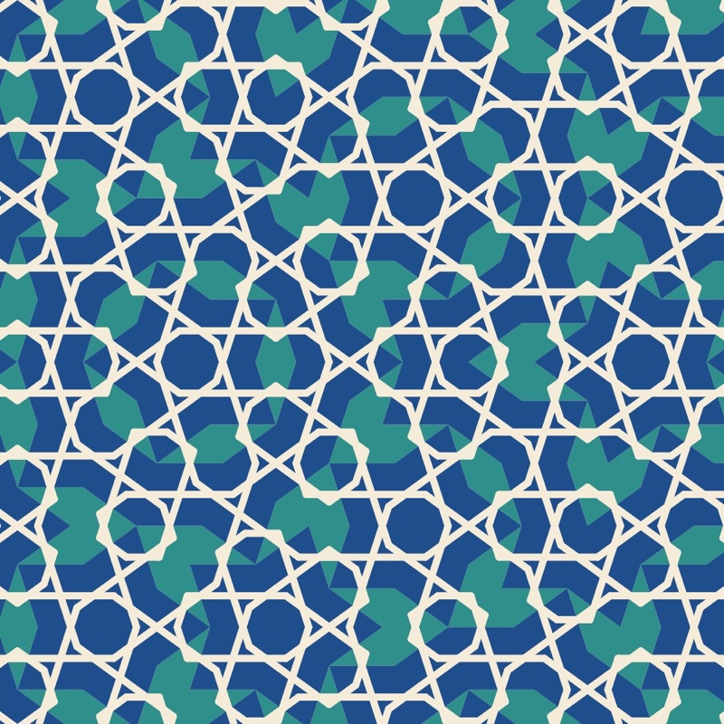
These tilings also have an artistic history. Girih, the interlaced-line decorations of Persian and Islamic architecture, are drawn on hidden tiles. Those of the Darb-i Imam shrine in Isfahan (1453) follow a Penrose tiling almost exactly, five centuries before Penrose (Lu and Steinhardt, Science, 2007).
In Laue
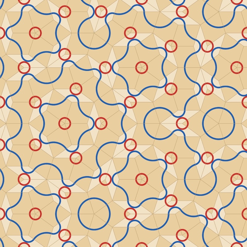
The workshop offers three tilings: Penrose (order 10), Ammann–Beenker (order 8) and dodecagonal (order 12), built from the grids or, for Penrose, by inflation (Built by). The Phason sliders move the cut. Perpendicular space shows where each vertex falls: hover over a vertex to find it there. The diffraction panel shows the peaks or the intensity map.
The Tiles section gives each kind of tile its own colour and sets the edges (zero hides them). The Decoration menu lays lines that run on from one tile to the next: the Penrose arcs, which draw its matching rules, arcs between the midpoints of the edges, ribbons that follow the de Bruijn lines, and girih strapwork at 36°, 54° or 72° to the edges. Design the Tiles… opens a tile in a large view so you can draw your own lines on it and place motifs. Everything you do there is repeated on every tile of the same kind, turned with it, and a stroke that ends on one of the marked points of the edges carries on into the neighbouring tile.
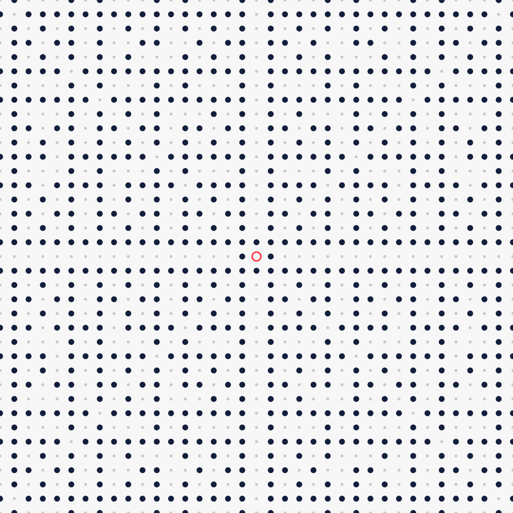
The Pattern menu also offers the visible points of the square or triangular lattice. Hover over a point to see its line of sight and the point that hides it. The k setting gives the k-free points, of which the visible points are the case k = 1.
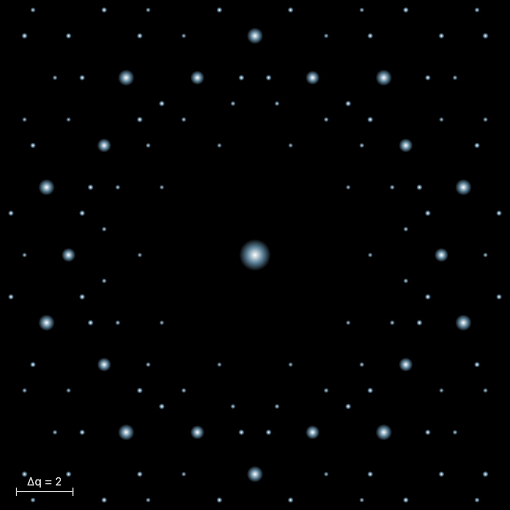
The Laue pattern
What the theory says
In 1912, Max von Laue had the idea of sending X-rays through a crystal. Walter Friedrich and Paul Knipping carried out the experiment, first on copper sulfate, then on zinc blende. Regularly arranged spots appeared on the photographic plate. The experiment proved two things at once: X-rays are waves, and a crystal is a lattice of atoms. Laue received the Nobel Prize in Physics in 1914.
The beam is white: it contains every wavelength of a band, and the crystal stays still. Each family of lattice planes makes an angle θ with the beam. From this spectrum it picks the wavelength that satisfies Bragg's law and sends it off in a direction deviated by 2θ, where it leaves a spot. The planes of one zone, parallel to a common axis, give spots lined up on an ellipse in transmission, and on a hyperbola in back-reflection.
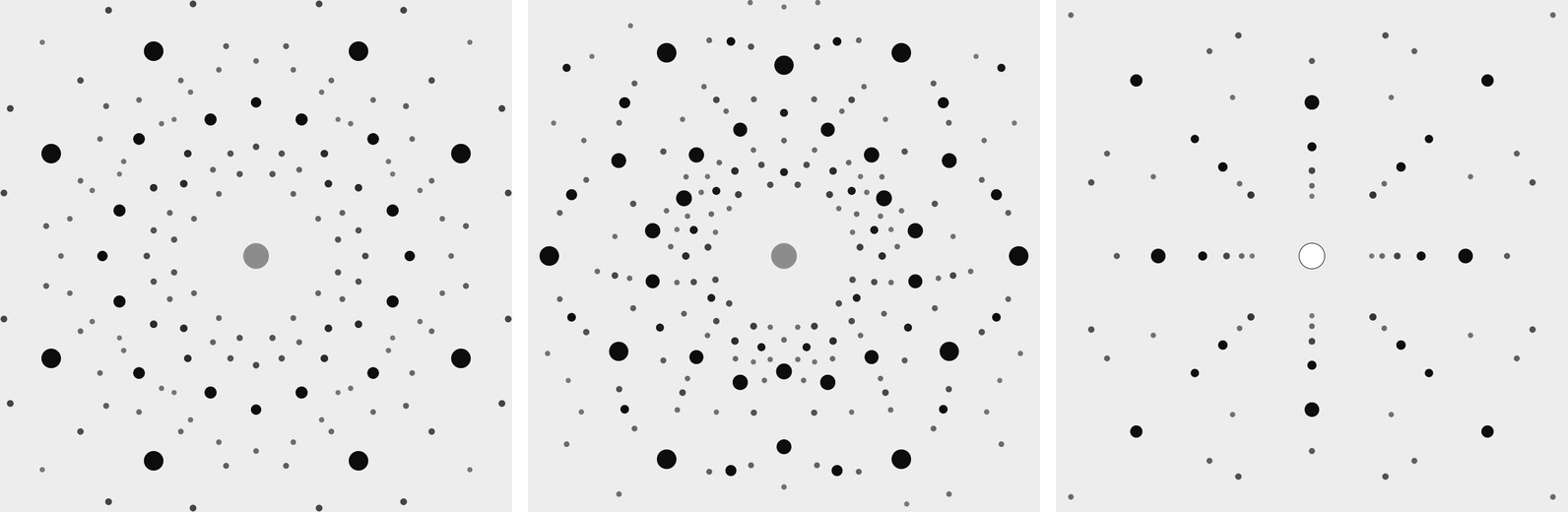
The arrangement of the spots shows the symmetry of the crystal seen along the beam. A four-fold axis parallel to the beam gives a pattern that repeats every quarter turn. Diffraction always adds a centre of symmetry (this is Friedel's law): the pattern therefore shows the Laue class, not the crystal class. This is the main use of the method: orienting a crystal before cutting it.
One spot gathers several harmonics. The planes (100), (200) and (300) send λ, λ/2 and λ/3 in the same direction. When the first reflection is extinguished, the spot still exists through the following ones.
From a spot to the planes
The pattern can also be read backwards: from a spot, you work back to the family of planes that produced it. Measure the position of the spot on the film, (x, y), and the distance D from the crystal to the film. The diffracted ray goes from the crystal to the spot; it makes the angle 2θ with the beam, with tan 2θ = r/D, r being the distance from the spot to the centre. Reflection obeys the mirror rule: the normal of the planes is the bisector of the angle between the incident beam and the diffracted ray. It therefore points along û − n̂, the difference between the unit vectors of the ray and of the beam. Its components along the axes a, b and c of the cell are proportional to the indices (h k l).
Take rock salt along [001], the film at 40 mm, and a spot at (0, 30) mm, with b pointing up on the film. Then û = (0, 30, 40)/50 = (0, 0.6, 0.8), n̂ = (0, 0, 1), and û − n̂ = (0, 0.6, −0.2), proportional to (0, 3, −1): these are the planes (0 3 1̄). Yet the F lattice extinguishes (0 3 1̄): the spot comes from its harmonic (0 6 2̄). The wavelength of each spot is not known: the Laue pattern gives the direction of the planes, that is, the orientation of the crystal, and not their spacings. In the laboratory, the spots are plotted on a stereographic projection, with the Leonhardt chart in transmission or the Greninger chart in back-reflection, and the angles between planes are recognised.
The formulas
Bragg's law picks the wavelength for each family of planes, with spacing , at the angle to the beam:
On a flat film at the distance from the crystal, in transmission, the spot lies at the distance from the centre:
From a spot (x, y), with the film at the distance , to the normal of the planes, then to their indices:
In Laue
In the Crystal workshop, Laue pattern (Diffraction tab) opens a panel above the stereogram. A white beam from 0.25 to 2.5 Å passes through the crystal along the direction of the view. The film is flat, 100 mm square, 40 mm from the crystal. The Film choice places it behind the crystal (Transmission, with a beam stop at the centre) or in front of it (Back-reflection, with the hole the beam passes through). When you turn the crystal, the spots move. The Look along buttons put an axis in the beam. The size and darkness of a spot follow its intensity, which adds up all the harmonics in the band. The panel's enlarge button opens the pattern in full: choose the radiation (X-rays with the tube voltage, or neutrons), the wavelength band and the film distance; zoom in, and pointing at a spot gives its indices, its harmonics, 2θ and d. The spots export as CSV. To check a calculation by hand, pointing at a spot in the enlarged pattern gives its indices. The exercises “The Laue pattern of salt” and “The Laue pattern of quartz” take you along this path step by step.
The powder pattern
What the theory says
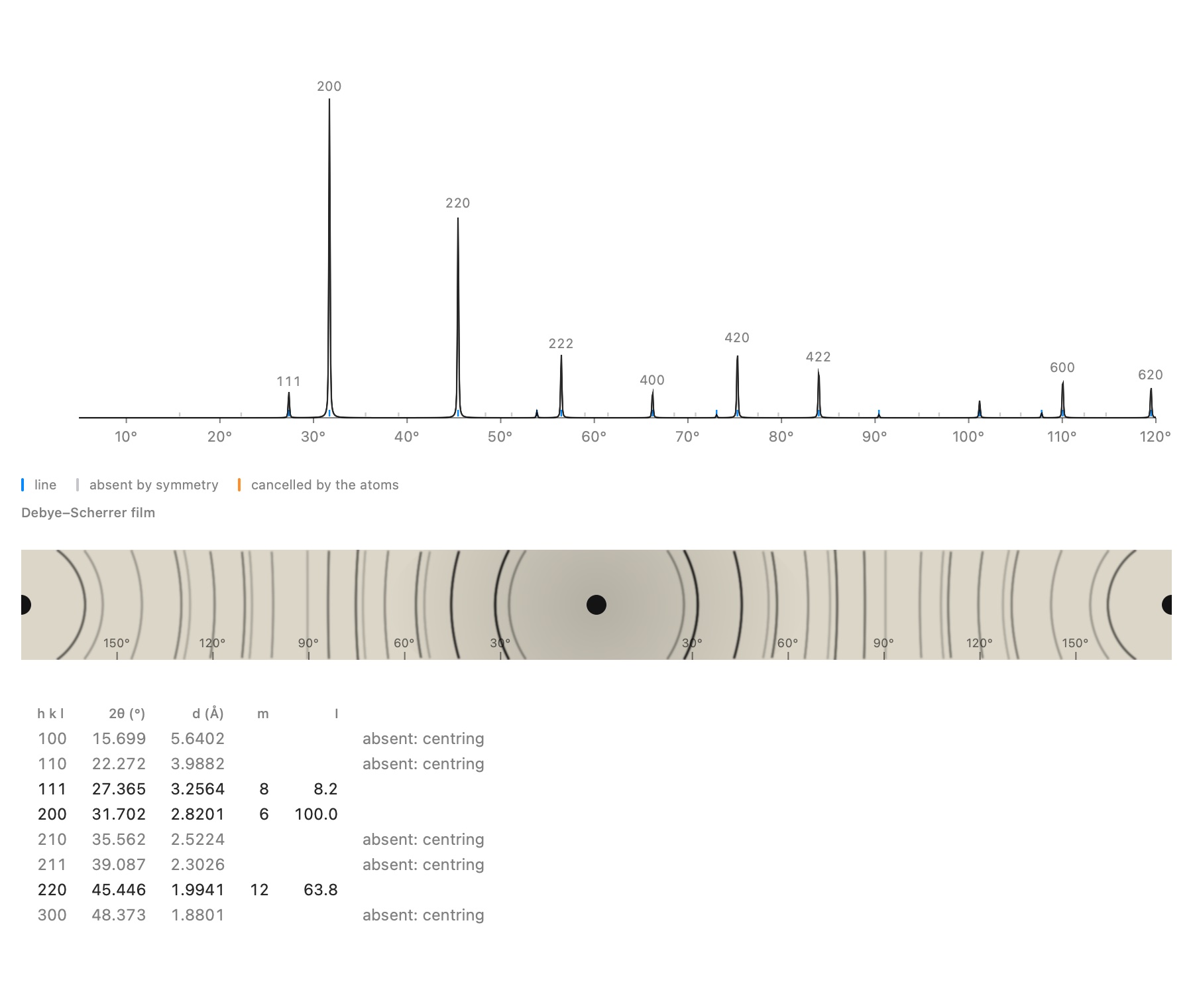
Most samples are not a single crystal but a powder: thousands of small crystals oriented at random. Each family of planes always finds a few well-oriented crystallites in it, so that each reflection becomes a cone around the beam, with half-angle 2θ. On a film wrapped around the sample, the Debye–Scherrer camera, each cone leaves a pair of arcs. A modern diffractometer measures the intensity as a function of 2θ: this is the powder pattern, the fingerprint of a crystalline phase.
A powder line gathers all the reflections with the same spacing d. Its intensity depends on several things:
- the structure factor;
- the multiplicity, that is, the number of equivalent reflections (six for 200 in a cubic crystal);
- a geometric factor, called the Lorentz-polarisation factor;
- the thermal motion of the atoms (the B factor), which weakens the high angles.
A line can be missing for two very different reasons. It can be extinguished by symmetry, whatever the atoms: a centring, a screw axis, a glide plane. It can also be cancelled by the atoms themselves, like the 222 line of diamond.
The formulas
The intensity of a powder line, with the multiplicity and the Lorentz-polarisation factor:
In Laue
In the Crystal workshop, Powder pattern (Diffraction tab) places the crystal's pattern below the view, recomputed whenever an atom moves. It is calculated with the atomic scattering factors of Waasmaier and Kirfel for X-rays, and with the coherent scattering lengths for neutrons. Enlarged, it shows its settings (radiation, wavelength, Kα₂ line, B, peak width, maximum 2θ), the table of lines and the Debye–Scherrer film. The table says why a line is missing: extinguished by the centring, a screw axis or a glide plane, or cancelled by the atoms. With Identical points, every atom scatters in the same way: only the lattice and the positions remain, and the odd lines of rock salt vanish, Na and Cl having become indistinguishable. The lines export as CSV, the curve as .xy.
A real powder measurement: refinement
What the theory says
A real measurement never looks quite like the calculation. The peaks have a width and a shape that depend on the instrument and on the sample; a background is added, and the zero of the instrument is slightly offset. With a copper anode, each line is also doubled by the Kα₂ line. The Rietveld method compares the measurement point by point with a calculated pattern, and adjusts the parameters until the discrepancy is as small as possible, by least squares. This yields a precise cell, often to within 10−4 Å, and proof that the model describes the sample well.
The profile of a line is modelled by a pseudo-Voigt function, a mixture of a Gaussian and a Lorentzian. Its width varies with angle according to Caglioti's law, and the background follows a Chebyshev polynomial. The quality is judged by two agreement factors: Rwp, the weighted discrepancy, and χ², which compares this discrepancy with the expected counting noise. A χ² close to 1 means that the model explains the measurement as well as the noise allows.
The formulas
The line width (Caglioti) and the minimised sum, with weights :
The agreement factors ( points, parameters):
In Laue
In the powder viewer, the Measurement section imports a file: two or three columns (2θ, intensity, standard deviation) as .xy, .xye, .dat or CSV, a powder CIF or a GSAS file. The measurement is overlaid on the calculation (the points, the calculated curve in red, the difference below). You choose the parameters to refine (scale, zero, sample displacement, background, widths, mixing, asymmetry, cell) and the 2θ range, then Refine runs the fit in two passes, in the background. Laue displays Rwp, χ² and the refined cell; Apply the cell writes it into the document. Laue has been validated this way on a real measurement of the NIST LaB₆ standard: the certified cell is recovered to within 3 × 10⁻⁴ Å.
An unknown powder: indexing
What the theory says
If you do not know what you have measured, you first need to find the cell: this is indexing, which assigns indices (h k l) to each line. For a cubic cell it is almost a game. The 1/d² values of the lines are in the ratios of the integers h² + k² + l², and the sequence of integers present even gives away the lattice. For lower symmetry, two or three parameters must be sought at once, and the number of possible solutions grows quickly. The quality of a solution is measured by de Wolff's figure of merit M₂₀: large when the lines fall exactly in place and few calculated lines remain unobserved. Once the cell is found, the missing lines point to the compatible space groups.
The formulas
For a cubic cell, and de Wolff's figure of merit (, lines calculated up to the 20th observed line, the mean discrepancy):
In Laue
The Indexing section of the viewer finds the peaks of the measurement (marked with orange triangles). It then looks for the cubic, tetragonal, hexagonal and orthorhombic cells that explain them, ranked by M₂₀. Monoclinic and triclinic cells are not searched for. For the chosen cell, Laue offers the compatible families of space groups, the most restrictive first. Use this cell and group writes them into the document, and refinement can begin.
Band structures
What the theory says
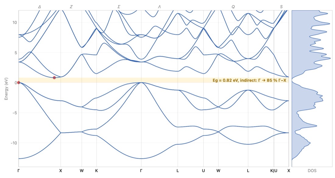
In an isolated atom, an electron is allowed only a few energy levels. In a crystal, an immense number of identical atoms come close together: each level broadens into a band, which holds as many states as there are cells. An electron in the crystal is a wave that travels through the whole lattice. Its state is labelled by a wave vector k, and its energy depends on k. Because the lattice repeats, it is enough to vary k within a single cell of the reciprocal lattice: the Brillouin zone.
The bands are drawn along a path that joins the high-symmetry points of the zone. These points have customary names: Γ at the centre, X at the middle of a square face, L at the centre of a hexagonal face. The lines that join them are named too: Δ from Γ to X, Λ from Γ to L, Σ from Γ to K.
Each band takes two electrons per cell, one of each spin. The bands are filled from the bottom up with the valence electrons:
- if the last full band is separated from the next by an empty interval, the band gap or forbidden band Eg, the crystal is an insulator (several eV, like salt) or a semiconductor (around 1 eV, like silicon);
- if a band is only partly filled, the electrons move without effort: it is a metal. The boundary between full and empty states is called the Fermi level.
The gap decides which light is absorbed. A photon whose energy exceeds Eg can lift an electron from the valence band to the conduction band; a less energetic photon passes through the crystal. The gap is direct when the top of the valence band and the bottom of the conduction band lie at the same k, as in gallium arsenide, at Γ. The crystal then absorbs and emits light well: LEDs and lasers are made from it. Otherwise the gap is indirect, as in silicon, from Γ to the line Δ: a vibration of the lattice, a phonon, is needed as well, and the crystal emits almost no light.
The formulas
The energy of a free electron, and the wavelength beyond which a crystal with gap no longer absorbs:
In Laue
In the Crystal workshop, Band structure (Properties tab) places a small band diagram beside the view, with the value of the gap or the word Metal. Enlarged, it shows the Brillouin zone in relief with its named points, the bands along the usual path and the density of states. For a semiconductor or an insulator, the Absorption tab gives the dielectric function, the refractive index, the absorption coefficient, the reflectivity and the Tauc plot. Three methods are offered:
- the empirical pseudopotential, fitted to optical measurements, for fourteen semiconductors with the diamond or zinc-blende structure (Si, Ge, GaAs, InP, ZnS…): the most faithful;
- tight binding, for any crystal that has atoms: a first look, metal or not, and the shape of the bands;
- the empty lattice, free electrons folded back into the zone, to understand where the bands come from.
Computed gaps often differ a little from measured ones. The Measured gap button raises the conduction bands to the measured value: these are the “scissors”. The bands, the density of states and the spectrum export as CSV, the graphs as images. The Silicon and Gallium arsenide examples open directly on their bands.
The scissors, in plain words: no band model gets the width of the band gap right (research calculations, by DFT, find it 30 to 50 % too small; tight binding sometimes too wide), but the shapes of the bands are good. The scissors cut the diagram in the middle of the gap and slide all the empty bands up or down, in one block, to the measured gap; nothing else changes. What this sets: the energy at which the crystal starts to absorb, hence its colour and its transparency, and its refractive index, which falls as the gap opens. The Gap correction (scissors) slider goes from −3 to +3 eV; Measured gap sets it when the value is known (the semiconductors of the pseudopotential, and some twenty common crystals in tight binding: diamond, rock salt, corundum, quartz, calcite, rutile…). The spectrum follows at once.
An alloy of two semiconductors from the table — Si₁₋ₓGeₓ, In₁₋ₓGaₓAs, GaAs₁₋ₓPₓ… — is computed as a virtual crystal: its form factors are the average of those of the two compounds, weighted by the fractions on the shared site. In the Construction tab, the Alloy section slides x from one to the other, the cell following Vegard's law. There you see the gap of GaAs₁₋ₓPₓ turn from direct to indirect (near x = 0.36; measured 0.45) and, in Si₁₋ₓGeₓ, the conduction valley of germanium take over from that of silicon (near x = 0.93; measured 0.85). The virtual crystal ignores disorder: it misses most of the gap bowing (In₀.₅₃Ga₀.₄₇As: 0.91 eV calculated, 0.75 eV measured), and it gives only one family of phonons where a real alloy has two.
A crystal that is not cubic does not have the same index in every direction: calcite doubles images because light polarised across its c axis sees the ordinary index nₒ = 1.658, and light polarised along it the extraordinary index nₑ = 1.486. The Polarisation menu of the Absorption tab shows the spectrum for E ⊥ c (ordinary), E ∥ c (extraordinary) or the Mean of the polarisations (three axes for a biaxial crystal). The Refractive index at 589 nm table sets the Measured row beside two models: Point dipoles, where each ion is deformed by the field of all the others, and Bands, with the gap correction, where the electrons move through the whole crystal. Laue marks as Recommended the one that came closest to the measurement for that kind of crystal: point dipoles for an ionic crystal with a wide gap (within 4 % for calcite, quartz, corundum, rock salt…), the bands below 5 eV (semiconductors, rutile); the bands, for their part, give the right sign of the birefringence nₑ − nₒ in all five uniaxial crystals tested.
Dispersion — the index changing with colour — shows on the Refractive index n, extinction κ curve: for the crystals whose dispersion has been measured (calcite, quartz, corundum, rutile, fluorite, rock salt, CsCl, zinc blende, diamond, SrTiO₃, silicon, GaAs), the Measured curve is drawn over it, dashed, for the polarisation chosen. The table of indices adds a V_d column, Abbe's number: the smaller it is, the more the crystal spreads white light into a rainbow (diamond 55, rutile 10, hence its “fire”). A last line gives the one-term Sellmeier formula of the recommended model, ready to paste into an optical design program; the Optical Spectrum (CSV)… export also holds the measured index. The model keeps Abbe's number within 20 % for 11 rays out of 14: to design optics, prefer the measured curve.
In a metal, the Fermi level crosses bands: the occupied states fill part of the Brillouin zone, and the Fermi surface separates them from the empty states. It is what decides conduction, the specific heat of the electrons and the response to a magnetic field. In the viewer, for a metal in tight binding or for free electrons (empty lattice), Fermi surface draws it in the zone, one colour per band, with below it its section by the plane through Γ across the view: turning the zone turns the section. The free electrons of copper give a sphere, entirely inside the zone; in tight binding it swells into necks that touch the eight hexagonal faces, at the L points, as Pippard's measurements showed (1957). For aluminium and its three electrons, the free sphere spills over into the second and third zones: this is Harrison's construction.
The vibrations of the crystal: phonons
What the theory says
The atoms of a crystal are not motionless: they vibrate about their positions, held by their bonds as if by springs. A vibration travels through the whole crystal as a wave, with wave vector q; its quantum is called a phonon. As for the electrons, it is enough to vary q within the Brillouin zone, and the frequency is drawn along the same path as the bands.
A crystal whose primitive cell contains N atoms has 3N branches:
- three acoustic branches, which start from zero at Γ: the whole cell moves as one block, and at long wavelengths these are the sound waves, one longitudinal and two transverse;
- 3N − 3 optical branches, in which the atoms of the same cell vibrate against one another. In an ionic crystal they carry a dipole and absorb infrared light.
In an ionic crystal, a longitudinal optical vibration also creates an electric field that stiffens it: its frequency (LO) exceeds that of the transverse vibrations (TO). The gap depends on the charges of the ions and on the screening by the electrons.
Stiff bonds and light atoms vibrate fast: diamond reaches 40 THz, rock salt stays below 8 THz. Phonons set the specific heat and the conduction of heat, and silicon needs them to cross its indirect gap.
The formulas
A chain of atoms of mass joined by springs of stiffness , with spacing :
In Laue
In the band-structure viewer, the Phonons tab draws the branches along the same path, with the vibrational density of states, in THz, cm⁻¹ or meV. For the tetrahedral semiconductors that Martin studied (Si, Ge, GaAs, InP…), the springs are those of Keating's model, fitted to the elastic constants. In an ionic crystal (rock salt, fluorite, perovskites…), the ions attract and repel one another through their charges: Laue adds these Coulomb forces, and near Γ the longitudinal optical branch rises above the transverse ones, as infrared measurements show. For the other crystals, Laue places universal springs between neighbours according to the nature of the bond (covalent or metallic), and holds the layers of graphite together. It is a first look at the branches, whose stiffness can be adjusted to compare with a measurement. A branch drawn below zero signals a structure that would rather deform: strontium titanate, cubic at room temperature, deforms in this way below 105 K.
Light and the crystal: infrared, Raman, birefringence
What the theory says
Visible light has a wavelength thousands of times larger than the cell: it sees the vibrations only at the centre of the Brillouin zone, at Γ. There are two ways of seeing them:
- infrared light is absorbed by a mode that sets an electric dipole vibrating, when ions of opposite charge move against each other;
- Raman scattering slightly changes the colour of a laser when a mode deforms the electron cloud, that is, the polarisability.
Symmetry decides which modes are active. In a crystal that has a centre of symmetry, a mode is never active in both infrared and Raman: this is the rule of mutual exclusion. The optical mode of silicon is seen only in Raman (520 cm⁻¹), that of rock salt only in infrared. Between the transverse frequency TO and the longitudinal one LO, an ionic crystal reflects almost all light: this is the reststrahlen band, “residual rays”, by which the far infrared was once isolated.
Symmetry also decides how visible light propagates. A cubic crystal has the same index in every direction. A tetragonal, trigonal or hexagonal crystal is uniaxial: light travelling along c is not split, any other ray separates into two, the ordinary and the extraordinary. The other crystals are biaxial. Calcite, with its flat, parallel CO₃ groups, is the most spectacular example: a line seen through a rhombohedron appears double.
The formulas
The dielectric function of an ionic crystal in the infrared, and the Lyddane–Sachs–Teller relation:
The colour of a gem most often comes from a trace: a colour centre in an otherwise perfect crystal. In ruby, a Cr³⁺ ion replaces about one aluminium in a hundred; the electric field of its six oxygens splits its d levels, and it absorbs yellow-green and violet: red remains. The same chromium in beryl, where this field is weaker, absorbs red: that is emerald. An electron trapped in a chlorine vacancy, an F centre, turns rock salt yellow.
In Laue
In the Crystal workshop, on the Properties tab, the Colour centres section adds a transition-metal ion in place of a cation (Cr³⁺, Ti³⁺, V³⁺, V²⁺, Fe²⁺, Co²⁺, Cu²⁺), an F centre on an anion site or a known band (blue sapphire, aquamarine, pink diamond, varieties of quartz). Laue derives from them the absorption bands, the transmitted spectrum and the colour seen in daylight; the optical density sets the thickness of the stone. The defect shows in the 3D view: the ion in its place, in the colour of its element and circled with dashes, or the empty vacancy with its electron. The examples Ruby, Emerald, Blue sapphire and Rock salt with F centres open set up this way.
When the bands have been measured in polarised light (ruby, blue sapphire), two swatches show the two colours of the crystal: light polarised perpendicular to the optic axis (E ⊥ c) and along the axis (E ∥ c). This is the dichroism that a dichroscope shows: ruby purplish red and orangy red, sapphire violetish blue and blue-green. Where the cross section of the ion has been measured (in corundum), Laue also gives the concentration, in atoms per million (ppma), that produces this optical density.
For ruby, the section also shows the Zeeman effect of the R lines, those of the ruby laser: in a magnetic field along the c axis, the ground level and the levels the lines start from split, and each line divides into components that fan out as the field grows, by about 8 cm⁻¹ at 10 teslas. Solid lines (σ) are seen in light polarised perpendicular to c, dashed ones (π) along c; their thickness follows their strength. It is through these fans that the levels of chromium in ruby were recognised.
In the band-structure viewer, the Infrared and Raman tab gives the modes at Γ, their degeneracy and what sees them (Infrared, Raman or Silent), the infrared reflectivity (for E ⊥ c and E ‖ c in a uniaxial crystal), the optical class and the indices in the visible, computed by the method of W. L. Bragg (1924). The tutor asks how many optic axes a crystal has.
Temperature: the atoms that vibrate
What the theory says
A crystal is never still. Each atom vibrates about its position, held by its bonds as if by springs. These vibrations break down into phonons, the waves of the Phonons section; at temperature T, each is the more strongly excited the smaller its energy hν is compared with k_BT. Even at 0 K, some agitation remains: the zero-point motion, imposed by quantum mechanics.
Several measurable quantities come from these vibrations. The specific heat C_v: at high temperature, each atom stores 3 k_B (the law of Dulong and Petit, 24.9 J/(mol·K) per mole of atoms); at low temperature, the modes freeze out one by one and C_v falls as T³ (Debye). The Debye temperature θ_D sums up the stiffness of the crystal in a single number: 343 K for copper, 645 K for silicon, over 2000 K for diamond. The mean square displacement ⟨u²⟩ of each atom weakens diffraction at high angles: this is the Debye–Waller factor, exp(−B sin²θ/λ²), with B = 8π²⟨u²⟩/3. Finally, by the Lindemann criterion, a solid melts when √⟨u²⟩ reaches 10 to 15 % of the distance between neighbours.
The formulas
In Laue
In the Crystal workshop, on the Simulations tab, the Temperature section gives the crystal a temperature. Thermal agitation sets it to 293 K; the slider and the field in kelvins adjust it, from 0 to 1500 K. It is saved with the document.
From the springs of the phonons, Laue derives the Debye temperature (the one that gives the same specific heat at this temperature, and its high-temperature value), the specific heat C_v, the B factor of each element and the Lindemann ratio, in orange when it exceeds 10 %. Two curves follow C_v and B from 0 to 1500 K, with the chosen temperature marked by a line.
This temperature is the same everywhere. The powder pattern and the Laue pattern then take the B of each element computed from the vibrations, instead of a single B: as the crystal heats up, the high-angle lines fade out. The Monte-Carlo of the spins (Magnetism section) also runs at this temperature.
Atoms vibrating in the 3D view sets the crystal in motion: each atom moves as the phonons dictate at this temperature, a sum of waves with randomly drawn phases. The motion is slowed down about a trillion times; the frequencies keep their ratios, and the optical modes run faster than the acoustic waves. As the crystal heats up, the agitation grows; at 0 K, the zero-point motion remains. Amplitude shows the motion as it is, or three or ten times larger to see it from a distance.
Displacement ellipsoids draws each atom as ORTEP does: the ellipsoid inside which it is found for a share of the time, 50 % by default as in papers; the Probability makes them all larger or smaller together, their shapes kept. Its axes are those of the atom's mean-square displacement tensor, averaged over the symmetry of its site: a sphere on a cubic site, an ellipsoid where the bonds leave the atom freer in one direction, as for the oxygens of quartz.
The same springs give the elastic constants of the crystal, derived from the speed of sound in forty directions, and its bulk modulus B. Together with the specific heat, they give the thermal expansion through the Grüneisen relation, α = γ C_v / (3 B V). The Grüneisen parameter γ says how much the vibrations stiffen when the crystal contracts; harmonic springs know nothing of it, and you enter it in the Grüneisen γ field, like the couplings of magnetism. It is 2 by default, as for most metals and ionic crystals; silicon has about 0.5. Laue shows α and the cell at this temperature, starting from 293 K, where a cell is usually measured; the powder pattern and the Laue pattern take this cell, and their lines shift as the crystal heats up.
The springs are those of the phonons: a first look, not a measurement. Copper gives θ_D = 321 K and B = 0.48 Ų at 300 K (measured: 343 K and 0.55 Ų), fluorite B = 0.44 Ų for calcium and 0.76 Ų for fluorine (0.47 and 0.68); silicon, whose transverse modes Keating's model stiffens, comes out a little too stiff. Its elastic constants, on the other hand, come back exactly: Martin fitted the springs to them. Those of copper and iron are too low (B = 101 and 100 GPa, against 137 and 170 measured): central springs between nearest neighbours cannot do better, and the expansion they give is too large in proportion.
Magnetism: spins and thermal agitation
What the theory says
Some ions carry a spin: their d electrons are not all paired. Mn²⁺ has five, all parallel (S = 5/2, Hund's rules), Ni²⁺ two (S = 1). Each spin is a small magnet. Between neighbours, the exchange J pushes them to line up (J positive, ferromagnetism) or to oppose each other (J negative, antiferromagnetism). Thermal agitation, for its part, disorders them. Above a critical temperature, T_C for a ferromagnet or T_N (Néel) for an antiferromagnet, it wins: the crystal is paramagnetic. Below it, an order sets in and grows on cooling.
The simplest model is the mean field of Weiss (1907): each spin sees of its neighbours only their average, as if it were a magnetic field. It gives the ordering temperature, the magnetisation that grows below it, the susceptibility χ that follows the Curie–Weiss law above it, and the jump of the specific heat at the transition. It neglects the fluctuations, which delay the order: it always overestimates the critical temperature, often by a third or a half.
The formulas
In Laue
In the Crystal workshop, on the Simulations tab, the Magnetism section places a moment on sites: Spins of the ions (Hund's rules) proposes S for each 3d transition-metal ion from its charge, and for the ferromagnetic metals (Fe, Co, Ni) an effective spin taken from the measured moment. Each site is up or down; the Propagation vector k (0, ½ or 1 on each axis) says how the sign changes from one cell to the next. The arrows of the spins appear in the 3D view.
Laue sorts the magnetic neighbours into shells (J₁, J₂…, with their distance and their number); you give J in meV for each. Couplings are measured, usually by inelastic neutron scattering; they are not computed here. Laue shows the mean-field ordering temperature, the Curie–Weiss θ and the effective moment. It also says whether another order of the same cell would appear first. Curves of temperature plots the order and the magnetisation, the susceptibility (parallel, perpendicular and powder) and its inverse, which crosses the axis at θ, and the specific heat.
The examples MnO, NiO and MnF₂ (antiferromagnets) and α-iron (a ferromagnet) come with published couplings and the measured temperature.
The mean field ignores fluctuations; Monte-Carlo shows them. Thermal agitation (Monte-Carlo) makes the spins of the 3D view tremble at the crystal's temperature, set in the Temperature section: well below T_N, the arrows oscillate around the order; nearing the transition, regions become disordered; above it, they point every which way. Below it, the sample's net magnetisation is shown live, in μ_B per atom and as a fraction of saturation, along with the order; a small graph places a point at each temperature where the temperature slider stops, on the mean field's curves: by moving it slowly across the transition, you trace for yourself the fall of iron's magnetisation, or the order of an antiferromagnet whose magnetisation stays zero. The simulated sample follows the view: as many magnetic cells per side as cells shown; when the view is filled, three crystal cells per side, or the whole view with the Phase transitions module. It is periodic at its edges. It is at least as large as the range of the couplings requires, so that a spin does not meet its own copy on the other side of the edge: seven cells for iron, whose couplings reach over ten shells of neighbours. In the curves window, the Monte-Carlo button heats thousands of spins from the order and places its points beside the mean field's curves. Its ordering temperature is lower, and closer to the measurement: MnF₂ orders near 70 K, against 87 K in mean field and 67 K measured.
A magnetic order has its own symmetry: the operations of the space group that bring each moment back onto itself, or onto its opposite if they are combined with time reversal 1′, which flips all the moments. They form a magnetic group, one of the 1651 Shubnikov groups. The Magnetism section names it in both notations of the tables, BNS and OG (MnF₂: P4₂′/mnm′; MnO: Cc2/c, where the c/2 translation of the doubled cell reverses the moments), and says in which directions each site can carry its moment. In the curves window, the neutron powder pattern shows what neutrons see, since they are sensitive to the moments: in colour, the magnetic lines, between those of the crystal for an antiferromagnet — the (½ ½ ½) of MnO, with which Shull and Smart discovered antiferromagnetism in 1949.
In an ordered magnet, a small deviation of one spin spreads to its neighbours as a wave: this is a spin wave, and its quantum is the magnon, as the phonon is the quantum of a vibration. In the curves window, Laue plots their energy along the path through the Brillouin zone, from the same couplings J. In a ferromagnet it starts from zero as k² (iron); in an antiferromagnet, as k (MnF₂, MnO). The Anisotropy D, which holds the moments on their axis, opens a gap at the bottom of the magnons. These are the curves measured by inelastic neutron scattering, and the source of the couplings in the examples.
Anisotropy also shows in a field. In the curves window, Laue plots the magnetisation M against the field B, at low temperature (5 % of the ordering temperature), with the field along the moments and across them. Across, the moments tilt gradually towards the field and M grows in a straight line. Along the moments, M first stays almost zero, then, at the spin-flop field, the moments turn all at once perpendicular to the field and M jumps onto the other line. Without anisotropy, the flop happens at the smallest field; the larger D, the later it comes. With D = 0.02 meV, MnF₂ flops near 9.5 T, against 9.27 T measured.
The magnetic group also says what the crystal can do. A net moment is allowed only if some direction stays fixed under all its operations: so it is in a ferromagnet, and in slightly canted antiferromagnets, the weak ferromagnets. The linear magnetoelectric effect, an electric field that magnetises the crystal, requires the group to break both inversion and time reversal. The Magnetism section says whether each is allowed, and gives the form of the magnetoelectric tensor α. The example of chromium oxide Cr₂O₃, ruby's antiferromagnetic cousin, is the textbook case: its group R-3′c′ contains neither inversion nor time reversal, but their product; α has two components there, a in the plane and b along c. Dzyaloshinskii predicted the effect in 1959 from this symmetry argument alone, and Astrov measured it the following year.
Phase transitions: broken symmetry, order and disorder
What the theory says
On cooling, many crystals change structure without melting. Barium titanate BaTiO₃, cubic above 393 K, becomes tetragonal: its titanium ions all shift to the same side and the crystal polarises; it is ferroelectric. In SrTiO₃, below 105 K, the TiO₆ octahedra rotate a little, alternately from one cell to the next. In β-brass, CuZn, copper and zinc occupy the sites of a body-centred cubic lattice at random above 741 K; below, the copper takes the corners and the zinc the centres. Each time, the low phase keeps only part of the symmetries of the high phase: its space group H is a subgroup of the high phase's group G. A transition is therefore read step by step in the list of the maximal subgroups of G, those that no other subgroup separates from it.
A subgroup loses either rotations or translations. If it keeps all the translations and loses rotations, it is translationengleiche (t): the cell stays the same, and the crystal splits into orientation domains, the twins, as many as the operations the point group has lost. If it keeps the rotations and loses translations, it is klassengleiche (k): the cell grows, and the crystal splits into antiphase domains, shifted by a lost translation. The index says how many operations are lost: 2 for CuZn going from Im-3m to Pm-3m, which loses the centring translation.
Landau (1937) describes the transition by an order parameter η, zero in the high phase and non-zero in the low phase: the polarisation of BaTiO₃, the angle of the octahedra of SrTiO₃, the difference in occupation of the two sites of CuZn. The free energy is expanded in powers of η, with only the terms the symmetry of the high phase allows. If a cubic term is allowed, the transition is first order: η jumps, as in Cu₃Au. Otherwise it can be continuous. A distortion breaks down into symmetry modes, each tied to an irreducible representation of the high group; the one that carries the order parameter says which instability drove the transition. Cochran (1960) linked it to the vibrations: as the transition approaches, the frequency of one phonon, the soft mode, falls towards zero, and its frozen shape is the low phase.
In an alloy, order comes from the energy of pairs of neighbours. Bragg and Williams (1934) gave its mean field: each site sees the average composition of its neighbours. As in magnetism, it ignores the fluctuations and overestimates the ordering temperature; Monte-Carlo keeps them. The specific heat and the susceptibility of the order peak at the transition, and the Binder cumulant goes from 2/3, in order, to 0. The same model describes the ions that enter a battery electrode: the cell's voltage is their chemical potential, and it takes a step where they order.
The formulas
In Laue
This chapter describes the Phase transitions module, opened by the subscription. In the Crystal workshop, Simulations tab, the Phase transitions section gives the maximal subgroups of the crystal's group: symbol, number, t or k and index. A click describes the chosen subgroup: its cell, its origin, its conjugates and the domains that form on cooling, orientations × translations. The k subgroups of index 2 to 4 are offered, those that enlarge the cell at most four times. Descend carries the crystal into the subgroup, in its standard setting: new cell, new origin, and each site that splits receives a number (Ti, then Ti_1 and Ti_2). It can be undone, the path taken stays shown above the list, and Back up returns one step.
Once down, move the atoms or type the positions of a measured structure: Laue measures the distortion from the highest group, in Å for each site. The Shown slider varies it in the 3D view, from 0% (the structure of the high phase) to 200% (the distortion enlarged). The distortion breaks down into symmetry modes, each with its wave vector (Γ, X, M, R…), its representation and its amplitude. Laue then names the order parameter: its representation, its dimension, the cubic and quartic invariants, and whether the transition can be continuous (Landau condition) and stay commensurate (Lifshitz condition). It also computes the phonons of the high phase, sorted by representation, and says whether the mode of the order parameter is the soft mode. With its springs, BaTiO₃ does find its polar mode unstable; in SrTiO₃ the model misses the instability of the octahedra, and Laue says so.
Landau–Devonshire opens the model of BaTiO₃ and PbTiO₃ with the published coefficients: the polarisation and the permittivity against temperature, the three transitions of BaTiO₃ (392, 283 and 202 K), the frequency of the soft mode by the Lyddane–Sachs–Teller relation, and the hysteresis loop at the chosen temperature.
For order–disorder, share a crystal's site between two elements (site inspector, Share this site with another element), then go down into a subgroup where this site splits: α-iron with Cu 50% and Zn 50%, towards Pm-3m (β-brass); copper with Cu 75% and Au 25%, towards Pm-3m of index 4 (Cu₃Au). The section then shows the order η, and Order–Disorder… opens the alloy's window. Give the transition temperature (the measured value is offered for CuZn, Cu₃Au, CuAu, FeCo and CuPd): Laue derives the ordering energy V from it, plots η by Bragg–Williams and by Monte-Carlo, and, by Monte-Carlo, the specific heat, the susceptibility and the Binder cumulant. The Monte-Carlo of CuZn orders near 0.8 of the mean-field temperature, as the Ising model predicts. High Resolution runs eight chains instead of two, with twice the points, for smoother curves. The T slider and Put This Order in the Crystal give each site the mean field's occupancy: the superstructure lines appear in the powder pattern, sharp for Cu₃Au, faint with X-rays for CuZn, whose two atoms have almost the same number of electrons.
The LiCoO₂ example opens the insertion voltage: when a crystal carries a mobile ion (Li, Na, Mg…), the section offers Insertion Voltage…. Each site is full or empty, with a repulsion V₁ between first neighbours and V₂ between second neighbours; a Monte-Carlo in which the ions come in and go out gives the voltage against the filling x, its derivative dx/dμ and the order in rows. The default values make the rows of lithium at x = ½ melt near 330 K, as measured, with a voltage step of about 0.1 V. The window also says what this simple model does not contain.
Finally, the module carries the large sample of the magnetic Monte-Carlo: the whole view filled with spins (see Magnetism).
Comparing with databases
What practice says
A model is only worth what its comparison with measurement shows. For many crystals, the accepted values are published in open databases: measured densities and indices, band gaps and dielectric constants calculated by density functional theory (DFT). These calculations are valuable but not infallible: their gaps are often 30 to 50 % too small. So you must always know whether a number was measured or calculated.
In Laue
In the Crystal workshop, on the Construction tab, the Reference values section opens a window that queries, only when you ask, Wikidata (measured densities and indices), refractiveindex.info (measured indices), AFLOW (calculated gaps and densities) and, with a free key, Materials Project (calculated gaps, densities, ε∞, ε(0) and indices). Laue sends only the formula and the space group number. Each value is shown with its nature (Measurement or Calculation), its source and a link, beside Laue's value.
The tutor
What teaching says
Symmetry is learned by handling it, and by getting it wrong. A useful exercise checks the answer and says why it is wrong. It gives hints without giving everything away, then shows the solution when you are stuck.
In Laue
The Exercises (Tutor) shelf has an audience selector (Design, Teaching, Science) and sorts the exercises by theme: first steps, plane groups, friezes, quasicrystals, lattices and densities, space groups and classes, Wyckoff positions, building structures, diffraction and absences, powder patterns, band structures.
A document from the Exercises (Tutor) shelf opens with the tutor panel: one instruction per step, a Check button and hints, one at a time. The engine does the checking: any equivalent position is right. A wrong answer is explained, for example “Na1 is on 8c (site symmetry -43m), not on 4a”, or, for a group, what the proposed group has more or less than the pattern. After a right answer, the solution explains why; once the hints run out, Show the solution shows it and lets you carry on. Some exercises hide the group or the symmetry elements, since finding them is up to you.
Printing and fabric
What the theory says
A pattern for printing must join without a seam: the right edge of one tile must continue exactly the left edge of the next. For a rectangular lattice, this is the straight repeat. For a centred or hexagonal lattice, the natural tile is offset from one row to the next: the half-drop drops each column by half a tile, and the half-brick shifts each row. Sharpness depends on resolution: 300 dots per inch for ordinary printing, more for fine textiles.
In Laue
Print or Fabric… exports the pattern alone, without cell or symbols, at a physical size: you set the cell edge in centimetres. The formats are vector PDF and SVG, sharp at any size, and PNG and TIFF at 150, 300 or 600 dpi, with the resolution written into the file. The background can be transparent. The size is a page (A4 to A2, Letter, Tabloid), a custom size or a seamless repeat: straight, half-drop or half-brick. For a print shop, the PDF gets 3 mm of bleed, crop marks and the sRGB profile. For screen printing, the separations give one film per colour, gathered in a ZIP. The SVG can have one layer per colour. The DXF, in millimetres, is for laser cutting and plotters. The Export menus also give the pattern's palette, for Adobe (ASE), GIMP and Inkscape (GPL) or Procreate. A mandala has its own print dialog, at its diameter in centimetres.
Printing a crystal in 3D
What the theory says
A model you hold in your hand is understood differently from a picture: you count the neighbours of an atom with your fingertip. A 3D printer lays down material layer by layer, from the bottom up. It asks for three things:
- a closed object, that is, a volume with no holes;
- a real size, in millimetres;
- an object that holds together: a thin spike breaks, an isolated atom falls off, and a part that leans by more than about 45° needs a support. The programs that prepare the print (PrusaSlicer, Bambu Studio, Cura, OrcaSlicer) add these supports themselves, as trees, suited to the printer and the material.
Two file formats dominate. STL is read everywhere, but it has neither colour nor unit. 3MF, the current format of the programs that prepare the print, keeps the millimetres, the colours and several parts in a single object. A printer with several materials can then give each element its own filament.
In Laue
In the Crystal workshop, 3D Print… opens the print dialog. There you choose:
- the format, 3MF or STL;
- the number of cells along a, b and c (one cell by default);
- the Longest side (mm) of the object;
- the Bond diameter (mm): 2.5 mm by default, with a warning below 2 mm.
Bonds that leave the object are never printed. Atoms that no bond holds are removed, unless you tick Keep the atoms no bond holds. Laue does not add supports: you ask the slicing program for them, and its tree supports suit a ball-and-stick model well.
The preview shows the object as it will be printed, sitting on the build plate, with the number of atoms and parts. If the object splits into several parts, adding cells is often enough to join them. Export… saves the file.
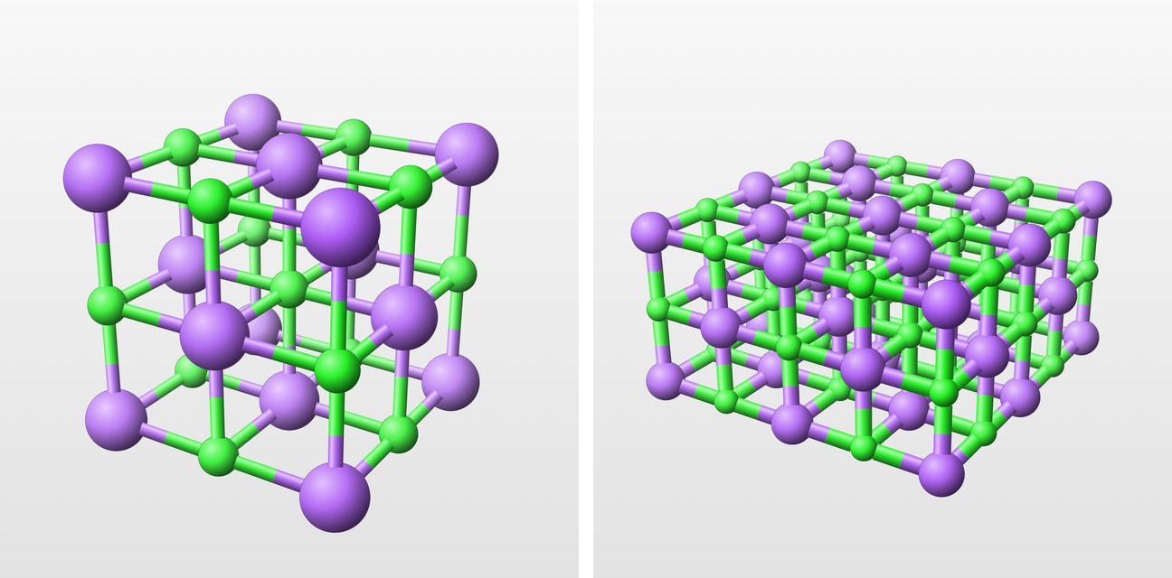
Presenting and exporting
In Laue
In the Crystal workshop, Save View keeps the orientation, the zoom and the display; saved views travel in the document. Present hides the panels and shows the views one after the other, with the arrow keys. Export Image saves the view as PNG, for a slide, or as vector PDF, for a paper or a handout, at the resolution set in the settings. The same menu saves a Turning Video (MP4): eight seconds in which the crystal turns once round on itself, about the cell axis nearest the vertical.